Download
1 / 40
400 likes | 579 Views
SIMULATION OF PARTIAL STRUCTURE FACTORS IN POLYISOPRENE. Departamento de Física de Materiales y Centro Mixto CSIC-UPV/EHU, Universidad del País Vasco, Apartado 1072, 20080 San Sebastián , Spain. People involved in this work:. From San Sebastián:. F. Alvarez, A. Arbe and J. Colmenero.

E N D
SIMULATION OF PARTIAL STRUCTURE FACTORS IN POLYISOPRENE Departamento de Física de Materiales y Centro Mixto CSIC-UPV/EHU, Universidad del País Vasco, Apartado 1072, 20080 San Sebastián , Spain
People involved in this work: From San Sebastián: F. Alvarez, A. Arbe and J. Colmenero From Jülich: S. Hoffman, L. Willner, R. Zorn, and D. Richter
INTRODUCTION: The structure of amorphous polymers at large scales seems to conform to a random coil model. However, little is known concerning more reduced scales at intermolecular levels. Partial static structure factors have been envisaged as a well established method for multicomponent systemsbut have hardly been used in polymer systems. (Spatial correlations in polycarbonates: Neutron scattering and Simulation), Journal Of Chemical Physics , 110, 3, 1819-1830 (1999) J. Eilhard and A.Zirkel, W.Tschöp, O. Hahn and K. Kremer, O.Schärpf, D.Richter and U.Buchenau.
INTRODUCTION: The static structure factor is defined as: For neutron scattering one can have the coherent static structure factor:
INTRODUCTION: neutron scattering by taking advantage of the different coherent scattering lengths of protons, deuteria and carbons: one can profit of selective labelling deuteration techniques in order to measure by neutron scattering the different contributions to the global static structure factor. Moreover, spin polarization analysis techniques can also be used in order to discriminate the coherent part out of the measurements.
INTRODUCTION: simulations From the spatial trajectories of all atoms in the system obtained by Molecular Dynamics Simulations, one can calculate both, the different total static structure factors and their separated partial contributions originating from the different species. The agreement between the calculations and the neutron scattering experiments is a confidence test to consider the separated contributions, which can only be obtained by simulations, as a useful tool to gain insight and knowledge about the structure and the dynamic behaviour of the different inner units in the system.
POLYISOPRENE: neutron scattering results Next we present the coherent static structure factors measured in the D7 spectrometer at the ILL in Grenoble at a temperature of 100 K for the following different deuterations: PIh8 fully protonated sample PId8 fully deuterated sample PId3 deuterated methyl groups PId5 all but the methyl groups deuterated
POLYISOPRENE: neutron scattering results Scoh(Q) Scoh(Q) PIh8 PId8 Q(Å-1) Q(Å-1) Scoh(Q) Scoh(Q) PId3 PId5 Q(Å-1) Q(Å-1)
cis-polyisoprene units 18% trans-polyisoprene units 82% POLYISOPRENE: molecular dynamics simulations Modeled microstructure
POLYISOPRENE: molecular dynamics simulations 100 monomer units Modeled microstructure
POLYISOPRENE: molecular dynamics simulations Periodic boundary conditions are imposed accordingly to the experimental density.
POLYISOPRENE: molecular dynamics simulations Simulation method: In order to perform the simulations the following modules from MSI (Molecular Simulation Inc. San Diego) were used: The model system was built by means of the AMORPHOUS CELL module. The simulations were run by using the INSIGHT (II 4.0.0. P version) and the DISCOVER-3 modules with the Polymer Consortium Force Field (PCFF).
POLYISOPRENE: molecular dynamics simulations Simulation method: Standard (conjugate-gradients) minimization procedures were applied in order to obtain a suitable starting point for a subsequent dynamics run at NVT conditions (T = 363 K) The Velocity-Verlet algorithm was used in order to numerically integrate Newton´s law of motion with a femtosecond time step, and the Velocity-Scaling algorithm was chosen to control the temperature Two consecutive dynamics runs were performed. The duration of the first one was of 1 nanosecond and the coordinate positions of all atoms were recorded every 0.01 picoseconds. The duration of the second was 2 nanoseconds and data were collected every 0.05 picoseconds.
POLYISOPRENE: molecular dynamics simulations From the coordinate positions of the atoms, one can calculate the van Hove function: which is related by means of a Fourier transform to the intermediate scattering function:
POLYISOPRENE: molecular dynamics simulations The van Hove function can be split into two contributions: The self part: and the distinct part:
POLYISOPRENE: molecular dynamics simulations If one assumes an isotropical averaging, one can also define the radial van Hove function (pair distribution function): so that gab(r,t) can be understood as the probability of finding a distance of r at time t among atoms of type a and those of type b. These gab(r,t) can be computed directly as histograms from the dynamic runs and Fourier transformed (weighted with their appropiate factors,ba and bb) in order to calculate any structure factor F(Q,t), namely, the static coherent one, Scoh(Q), which can be directly compared to the experimentally measured ones.
POLYISOPRENE: comparison between MD and NS results Scoh(Q) Scoh(Q) PIh8 PId8 Q(Å-1) Q(Å-1) Scoh(Q) PId3 PId5 Q(Å-1) Q(Å-1)
POLYISOPRENE: comparison between MD and NS results Scoh(Q) Scoh(Q) PIh8 PId8 Q(Å-1) Q(Å-1) Scoh(Q) PId3 PId5 Q(Å-1) Q(Å-1)
POLYISOPRENE: comparison between MD and NS results Neutron scattering result from a measurement at 100 K at the D20 instrument in Grenoble compared to MD calculation. Scattered intensity (barn/srad/atom) PId8
POLYISOPRENE: the dynamic case Once the comparison with experiments has shown favourable as a confidence test to trust the simulations, one could go a step further and calculate the (partial) dynamic structure factors. As an example of the latter we will show some results that can shed some light for a better understanding of Neutron Spin Echo (NSE) measurements performed in polyisoprene: - about the range of validity of the traditional analysis in the fully deuterated sample, PId8. - about a qualitative understanding of results in a partially deuterated sample, PId5.
POLYISOPRENE: the dynamic case First, let us recall that what it is measured by NSE is the following magnitude:
POLYISOPRENE: the dynamic case Merging of the a and b relaxations in PB: A neutron spin echo and dielectric study. A Arbe, D. Richter, J. Colmenero and B. Farago, Physical Review E, 54, 4 (1996)
Iinc Scoh(Q) NSE 1.3 2.3 0.8 POLYISOPRENE: the dynamic case PId8, t = 0
POLYISOPRENE: the dynamic case PId8, Q = 0.8 Icoh(0.8,t) Icoh(0.8,t)- Iinc(0.8,t)/3 -Iinc(0.8,t)/3
POLYISOPRENE: the dynamic case PId8, Q = 1.3 Icoh(1.3,t) Icoh(1.3,t)- Iinc(1.3,t)/3 -Iinc(1.3,t)/3
POLYISOPRENE: the dynamic case PId8, Q = 2.3 Icoh(2.3,t) Icoh(2.3,t)- Iinc(2.3,t)/3 -Iinc(2.3,t)/3
Icoh(Q,t) Icoh(Q,t)- Iinc(Q,t)/3 0.8 POLYISOPRENE: the dynamic case <tKWW> values obtained from fittings to a Kohlrausch-Williams-Watts function
POLYISOPRENE: the dynamic case PId5 Q=1.09 Å-1 Q=1.27 Å-1
Iinc Scoh(Q) NSE POLYISOPRENE: the dynamic case PId5, t = 0
POLYISOPRENE: the dynamic case PId5, Q = 0.8 Icoh(0.8,t) Icoh(0.8,t)- Iinc(0.8,t)/3 -Iinc(0.8,t)/3
POLYISOPRENE: the dynamic case PId5, Q = 1.3 Icoh(1.3,t) Icoh(1.3,t)- Iinc(1.3,t)/3 -Iinc(1.3,t)/3
POLYISOPRENE: the dynamic case PId5, Q = 2.0 Icoh(2.0,t) Icoh(2.0,t)- Iinc(2.0,t)/3 -Iinc(2.0,t)/3
POLYISOPRENE: the dynamic case Q=1.09, measured Q=1.27, measured PId5
POLYISOPRENE: the dynamic case Q=1.1, simulation Q=1.09, measured Q=1.3, simulation Q=1.27, measured PId5
Icoh(Q,t) Icoh(Q,t)- Iinc(Q,t)/3 POLYISOPRENE: the dynamic case bKWW values obtained from fittings to a Kohlrausch-Williams-Watts function