Objective
Characterization of the Ozone and Transport Conditions During the Four OTAG Episodes Bret A. Schichtel and Rudolf B. Husar Center for Air Pollution Impact and Trend Analysis (CAPITA) Washington University St. Louis, Missouri Presented at A&WMA's 91st Annual Meeting June 14 -18, 1998.

Objective
E N D
Presentation Transcript
Characterization of the Ozone and Transport Conditions During the Four OTAG Episodes Bret A. Schichtel and Rudolf B. Husar Center for Air Pollution Impact and Trend Analysis (CAPITA) Washington University St. Louis, MissouriPresented at A&WMA's 91st Annual MeetingJune 14 -18, 1998
Objective Establish qualitative relationships between measured ozone levels and synoptic scale meteorological and transport conditions for each OTAG episode. Assess the extend of regional scale transport of elevated ozone Concentrations. Method • Data Fusion - Concurrently visualize ozone, meteorological and transport data by animating walls of data for each episode.
OzoneData OTAG Domain
Meteorological Data National Meteorological Centers Nested Grid Model (NGM) Time range:1989 - 6/97 Horizontal resolution: ~ 160 kmVertical resolution: 10 layers up to 7 km3-D variables:u, v, w, temp., humiditySurface variables include: Precip, Mixing Hgt,….
Figure 2. The measure 2 PM ozone concentrations for every third day in the 1988 OTAG Episode as point data and as contours.
Figure 3. The average daily maximum ozone for the A) 1988, B) 1991, c) 1993, d) 1995 and e) aggregated ’88, ‘91, ‘93, ‘95 OTAG Episodes.
Figure 4. The 2 PM measured ozone and NGM meteorological data for every second day of the 1991 OTAG episode. The six panels from left to right are: Measure ozone point data, measured ozone contoured, three day back trajectories, precipitation field, temperature field at ~150 meters above the surface, and wind vectors at ~150, 500, and 900 meters above the surface.a.
Figure 5. The 2 PM measured ozone and NGM meteorological data for every second day of the 1993 OTAG episode starting on July 23rd. The six panels from left to right are: Measure ozone point data, measured ozone contoured, three day back trajectories, precipitation field, temperature field at ~150 meters above the surface, and wind vectors at ~150, 500, and 900 meters above the surface.a.
Figure 6. The 2 PM measured ozone and NGM meteorological data for every second day of the 1995 OTAG episode. The six panels from left to right are: Measure ozone point data, measured ozone contoured, three day back trajectories, precipitation field, temperature field at ~150 meters above the surface, and wind vectors at ~150, 500, and 900 meters above the surface.a.