Download
1 / 55
550 likes | 667 Views
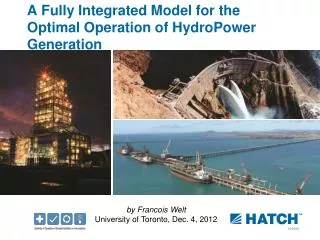
A Fully Integrated Model for the Optimal Operation of HydroPower Generation. by Francois Welt University of Toronto, Dec. 4, 2012. Hatch Power and Water Optimization Group. Engineering Company Specialized group within Hatch Renewable Power Experience: Over 40 systems implemented

E N D
A Fully Integrated Model for the Optimal Operation of HydroPower Generation by Francois Welt University of Toronto, Dec. 4, 2012
Hatch Power and Water Optimization Group • Engineering Company • Specialized group within Hatch Renewable Power • Experience: • Over 40 systems implemented • Experience with different types of hydro systems • Supported by over 9,000 multi-disciplinary engineering professionals worldwide
Hatch Power and Water Optimization • Water Resource and Power System Modeling – Simulation and Optimization • System Implementation • Configuration, Test • Integration / Communications • Install and Train • Studies • Asset Management / Life cycle analysis • Wind Farm Design Optimization
Hydro Optimization in Generation PlanningConcepts • Make best use of limited hydro resources • Meet operational constraints • Maximize Profits • Maximize sales/ Minimize costs • Calculate optimal plant/unit MW • Calculate optimal WL trajectory/ spill releases • Calculate bid curve Optimization technologies becoming increasingly attractive with improvements in computing speeds/ capabilities
Optimization Statistics Examples of potential economic benefits from optimization - Short term operation Ref: “Assessing the Economic Benefits of Implementing Hydro Optimization”, Hydro Review magazine, 1998 Typically, potential improvements between 1 – 5%
Hydro OptimizationTime Scale Plant/ units Smaller reservoir Larger reservoir • Long Term (LT): • Generation/Water Plan • Targets and Water Values • Short Term (ST): • Schedule • Transactions Real Time (RT): Dispatch To end of week/month To end of water year Hour/day end/
Optimization Problem • Must formulate problem in terms of: • Objective functions • Constraints • Rules of operation • Physical relations • Decision Variables • Characteristics: • One set of decisions per time step, piece of equipment • Hydraulic network • Transmission network • Large problem size
Physical Representation • Hydraulic Network • Source: Inflow Points • Sink: downstream outlet • Water conveyance/ Flow • Storage • Head (Potential energy) and head loss • Can be bi-directional (gen/pump) • Electric Network • Source: Generation points • Sink: Load or Market points • Bi-directional • Energy losses
Hydro System Components Inflow Arc River Reach Reservoir Node Spill Arc Power Arc Tailwater Junction Node River Reach
8 8 8 8 8 8 8 8 8 8 8 8 8 8 8 8 8 8 Rock Island Schematic Powerhouse Two Powerhouse One Spillway F F F
Hydraulic Network Representation • Continuity equation at each reservoir node Σ Qin – ΣQout = V(t) – V(t-1) • Continuity equation at each junction node Σ Qin – ΣQout = 0 • Conveyance in reach arc Qout (t) = Σα(n).Qin(t-n)
D H X X T Transmission Area Transaction Load Demand Committed Transactions Hydro Generation • Market • Purchase • Sale • Bilateral • Purchase • Sale Thermal Generation Wind Generation Wind
X(COB1) S W MW X(COB1) P X(PNW1) S X(COB2) S X(PNW1) COB2S Plant 4 COB3P P P P P P X(PSE) X(PNW2) X(MIDC) X(PNW3) X(COB3) S X(BPA-X) S X(PSE) X(MIDC) X(PNW2) X(PNW3) “aggregate unit” Contract Bus COB2P Supply Area River 1 BPA1 X(COB2) P Plant 1 Bus A COB1 Bus Configuration Plant 2 PSE Bus B X MW Y MW S L River 2 Plant 3 BPA2 Z MW S “line limits” S River 3 X(COB3) BPA3 P MID-C Plant 5 “group line limits” S COB3S Plant 6
Network Representation • Electric Network • Continuity equation at node (bus) Σ MWin – ΣMWout = 0 • Losses through conveyance (tieline) MWout = Mwin - α.Mwin^2 • MW Energy • MW ancillary service (reserve)
NON-SPINNING OPERATING RESERVE NON_AGC MAX MW TOTAL SPINNING LOAD FOLLOW. SPINNING AGC (Regulating) CONTROL MW GENERATION Physical RepresentationReserves and Generation • Unit/Plant Balance Equation REG Down
Joint Optimization • Energy and A/S markets with price forecasts • Optimal trade-off between energy and A/S • Spin • Non Spin • Regulation Up • Regulation Down Energy • Unused capacity can earn revenues with resulting unused water still sold as energy at a later date • Some of the unused capacity can be converted into energy when reserve is called (Take)
Physical Relations: Plants and Units • Power-flow-head relationship (3-D)
Spillway Equations Q = Co ·Le ·Open·(hwl - E)Eo E = Esill or twl hwl Submerged Flow Free Overflow ESill hwl twl ESill Q = Cf ·Le ·(hwl - Esill)Ef
Operational Constraints Representation • Hydraulic Constraints • Simple Constraints on Flow, storage (WL), MW • Time aggregated constraints (linear) • Max average • Max/min between periods • Relational constraints (including step functions) • Electric Constraints • Simple Max/ Min on generation • Tieline flow (congestion) • Reserve (min/max)
Complexities in Formulation • Uncertainty • Inflow • Load • Market price • Hydraulics • Non-linear physical constraints • generation with cross product (flow * head^a) • Losses (quadratic) • Spill representation • Spatial/time connectivity • Discreteness • Start/stop costs • Spinning reserve • Non continuous operating range • Large Scale • Time dependent decisions (up to 200,000 decision variables / constraints) Long Term Short Term Real Time
Preferred Schemes for Hydro • Plants are hydraulically and electrically connected • Water conveyance • Load, reserve • Fixed amount of water over time – strong temporal interdependency • Decomposition • Subproblems • Bender’s cuts • Dynamic Programming • Nonlinear Programming • Linear Programming • Piecewise linearization • Successive Linearization • Semi-heuristics
Long Term Model Principles • Consideration for Future Uncertainty • Stochastic • Detailed Physical Representation • Simplified Time Definition • Periods (week(s), month) • Sub-period (peak, off-peak, weekend,…) • Time Average answers • Based on scenario analysis – consider all cross correlations
LT Vista Mathematical Model • Electric network: • Buses • tielines Hydraulic network: • arcs (plant, spill, river reaches) • nodes (reservoirs, junctions) Inputs: - hydraulic: stochastic inflow, start/end WL - electric: transactions, load Engine Stochastic SLP (2 stage) Detailed Plant Operation Detailed constraint set Benders Decomposition Constraints: - hydraulic (flow, elevation, etc.) - electric (transmission, etc.)
LT Vista Methodology • Two Stage LP • Decomposition Master 1st Period / Future period subproblem Future 1 Future 2 NOW Future 3 Future N
LT Vista Methodology • Multi-dimensional Uncertainty -- Inflow, Market and Load Load Market H1_M2_L1_ Hydrology H1_M1 H1_M2_L2 H1_M2 H1 H1_M2_L3 H1_M3 H1_M2_Ll H1_Mm
LT Vista Time Definition • Period: • basic model time step (e.g., 1 week) • SubPeriod: • Peak-off peak (Load duration) aggregation within periods • Time blocks • constraints tying several periods/subperiods subperiods period Time block
Short Term Model Principles • Deterministic Model • Detailed Physical Representation • Detailed Hourly Time Definition • SLP numerical scheme with piecewise representation: • MW/Flow relation • Tieline losses • Unit Dispatch/Unit Commitment Subproblem • Nonlinear Programming • DP • Spinning reserve allocation subproblem • Integrated handshake with Long Term Model • Market Analysis
Unit Dispatch/ Unit Commitment Subproblem • Plant Representation based on optimal unit dispatch/ unit commitment around base solution • Plant Generation function used in SLP • Best Dispatch answers used in scheduling • General LP problem formulation cannot deal with discrete decisions – unit ON or unit OFF • Unit Dispatch • Model • Snapshot Non linear analysis • Fixed Head Plant 1 Non continuous operation Plant 2 Plant N
Spill Allocation • Aggregated spill representation • Piecewise linear representation • No flow zone • Sequencing issues – heuristic vs integer set • Stability issues Spill 1 Spill 2 Spill N
LT – ST Handshake • Type • Economic • Seasonal Reservoirs: Value of water in storage applied to end of opt period water levels • Other Reservoirs/head ponds: Max Target Water Levels at the end of opt period. • Target Water Levels • Seasonal Reservoirs: LT Target Levels applied to end of opt period water levels • Other Reservoirs/head ponds: Max Target Water Levels at the end of opt period • Target Flow Releases • Seasonal Reservoirs: LT Target Levels applied to end of opt period water levels • Other Reservoirs/head ponds: Max Target Water Levels at the end of opt period • Others • meet target water levels defined by user • Custom • Combination of above
Spinning Reserve Allocation Subproblem • Linearized formulation of spinning reserve • Subproblem is to find best unit allocation to meet spinning reserve requirements • LP Unit representation
4 hr 2 hr 8 hr Total Bus Generation: Comparison between Time Groupings
ST Vista Run Times (866 MHz) Day Ahead Study Period
MW Flow Semi-Heuristic Resolution Schemes • Plant retirement/commitment • Plant zone resolution • Uncontrolled spillway structure • Semi-heuristic – does not cover all solution space • Perturbation to the LP global problem
Future MW Base Storage Dev Time Price-Volume CurvesMethodology • Cost sensitivity calculation $ MWh
Real Time Model Principles • Deterministic Model • Detailed Physical Representation • Detailed sub hourly Time Definition • Detailed Unit Dispatch/Unit Commitment Sub-problem • Integrated handshake with Short Term Model