Download
1 / 17
170 likes | 216 Views
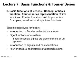
Lecture 7: Basis Functions & Fourier Series. 3. Basis functions (3 lectures): Concept of basis function. Fourier series representation of time functions. Fourier transform and its properties. Examples, transform of simple time functions. Specific objectives for today:

E N D
Lecture 7: Basis Functions & Fourier Series • 3. Basis functions (3 lectures): Concept of basis function. Fourier series representation of time functions. Fourier transform and its properties. Examples, transform of simple time functions. • Specific objectives for today: • Introduction to Fourier series (& transform) • Eigenfunctions of a system • Show sinusoidal signals are eigenfunctions of LTI systems • Introduction to signals and basis functions • Fourier basis & coefficients of a periodic signal
Lecture 7: Resources • Core material • SaS, O&W, C3.1-3.3 • Background material • MIT Lecture 5 • In this set of three lectures, we’re concerned with continuous time signals, Fourier series and Fourier transforms only.
Why is Fourier Theory Important (i)? • For a particular system, what signals fk(t) have the property that: • Then fk(t) is an eigenfunction with eigenvaluelk • If an input signal can be decomposed as • x(t) = Sk akfk(t) • Then the response of an LTI system is • y(t) = Sk aklkfk(t) • For an LTI system, fk(t) = est where sC, are eigenfunctions. x(t) = fk(t) y(t) = lkfk(t) System
Why is Fourier Theory Important (ii)? • Fourier transforms map a time-domain signal into a frequency domain signal • Simple interpretation of the frequency content of signals in the frequency domain (as opposed to time). • Design systems to filter out high or low frequency components. Analyse systems in frequency domain. Invariant to high frequency signals
Why is Fourier Theory Important (iii)? • If F{x(t)} = X(jw) w is the frequency • Then F{x’(t)} = jwX(jw) • So solving a differential equation is transformed from a calculus operation in the time domain into an algebraic operation in the frequency domain (see Laplace transform) • Example • becomes • and is solved for the roots w (N.B. complementary equations): • and we take the inverse Fourier transform for those w.
Introduction to System Eigenfunctions • Lets imagine what (basis) signals fk(t) have the property that: • i.e. the output signal is the same as the input signal, multiplied by the constant “gain” lk(which may be complex) • For CT LTI systems, we also have that • Therefore, to make use of this theory we need:1) system identification is determined by finding {fk,lk}. • 2) response, we also have to decompose x(t) in terms of fk(t) by calculating the coefficients {ak}. • This is analogous to eigenvectors/eigenvalues matrix decomposition x(t) = fk(t) y(t) = lkfk(t) System x(t) = Sk akfk(t) y(t) = Sk aklkfk(t) LTI System
Complex Exponentials are Eigenfunctions of any CT LTI System • Consider a CT LTI system with impulse response h(t) and input signal x(t)=f(t) = est, for any value of sC: • Assuming that the integral on the right hand side converges to H(s), this becomes (for any value of sC): • Therefore f(t)=est is an eigenfunction, with eigenvalue l=H(s)
Example 1: Time Delay & Imaginary Input • Consider a CT, LTI system where the input and output are related by a pure time shift: • Consider a purely imaginary input signal: • Then the response is: • ej2t is an eigenfunction (as we’d expect) and the associated eigenvalue is H(j2) = e-j6. • The eigenvalue could be derived “more generally”. The system impulse response is h(t) = d(t-3), therefore: • So H(j2) = e-j6!
Example 1a: Phase Shift • Note that the corresponding input e-j2t has eigenvalue ej6, so lets consider an input cosine signal of frequency 2 so that: • By the system LTI, eigenfunction property, the system output is written as: • So because the eigenvalue is purely imaginary, this corresponds to a phase shift (time delay) in the system’s response. If the eigenvalue had a real component, this would correspond to an amplitude variation
Example 2: Time Delay & Superposition • Consider the same system (3 time delays) and now consider the input signal x(t) = cos(4t)+cos(7t), a superposition of two sinusoidal signals that are not harmonically related. The response is obviously: • Consider x(t) represented using Euler’s formula: • Then due to the superposition property and H(s) =e-3s • While the answer for this simple system can be directly spotted, the superposition property allows us to apply the eigenfunction concept to more complex LTI systems.
History of Fourier/Harmonic Series • The idea of using trigonometric sums was used to predict astronomical events • Euler studied vibrating strings, ~1750, which are signals where linear displacement was preserved with time. • Fourier described how such a series could be applied and showed that a periodic signals can be represented as the integrals of sinusoids that are not all harmonically related • Now widely used to understand the structure and frequency content of arbitrary signals w=1 w=2 w=3 w=4
Fourier Series and Fourier Basis Functions • The theory derived for LTI convolution, used the concept that any input signal can represented as a linear combination of shifted impulses (for either DT or CT signals) • We will now look at how (input) signals can be represented as a linear combination of Fourier basis functions (LTI eigenfunctions) which are purely imaginary exponentials • These are known as continuous-time Fourier series • The bases are scaled and shifted sinusoidal signals, which can be represented as complex exponentials x(t) = sin(t) + 0.2cos(2t) + 0.1sin(5t) ejwt x(t)
Periodic Signals & Fourier Series • A periodic signal has the property x(t) = x(t+T), T is the fundamental period, w0 = 2p/T is the fundamental frequency. Two periodic signals include: • For each periodic signal, the Fourier basis the set of harmonically related complex exponentials: • Thus the Fourier series is of the form: • k=0 is a constant • k=+/-1 are the fundamental/first harmonic components • k=+/-N are the Nth harmonic components • For a particular signal, are the values of {ak}k?
Fourier Series Representation of a CT Periodic Signal (i) • Given that a signal has a Fourier series representation, we have to find {ak}k. Multiplying through by • Using Euler’s formula for the complex exponential integral • It can be shown that T is the fundamental period of x(t)
Fourier Series Representation of a CT Periodic Signal (ii) • Therefore • which allows us to determine the coefficients. Also note that this result is the same if we integrate over any interval of length T (not just [0,T]), denoted by • To summarise, if x(t) has a Fourier series representation, then the pair of equations that defines the Fourier series of a periodic, continuous-time signal:
Lecture 7: Summary • Fourier bases, series and transforms are extremely useful for frequency domain analysis, solving differential equations and analysing invariance for LTI signals/systems • For an LTI system • est is an eigenfunction • H(s) is the corresponding (complex) eigenvalue • This can be used, like convolution, to calculate the output of an LTI system once H(s) is known. • A Fourier basis is a set of harmonically related complex exponentials • Any periodic signal can be represented as an infinite sum (Fourier series) of Fourier bases, where the first harmonic is equal to the fundamental frequency • The corresponding coefficients can be evaluated
Lecture 7: Exercises • SaS, O&W, Q3.1-3.5