Download

1 / 43
430 likes | 534 Views
Plots, Graphs, and Sketches (1.1). Plots or Graphs - Generally the most effective format for displaying and conveying the interrelation of experimental variables.

E N D
Plots, Graphs, and Sketches (1.1) • Plots or Graphs - Generally the most effective format for displaying and conveying the interrelation of experimental variables. • Sketches - Quick and informal method of sharing ideas with others or clarify concepts for yourself. Free body diagrams (FBDs) are an example.
Plots and Graphs • Means of Communicating Ideas Concisely • Axes • X-axis (horizontal, independent variable) • Y-axis (vertical, dependent variable) • Divide major axes into appropriate divisions of 1, 2, 10, 10X, etc • Label with words, symbols, and units • Minor axes should be distributed evenly
Sections 1.2 • Functions: • Independent variables (Cause /Input /Action) • Dependent variables (Effect /Output / Reaction)
Dependent / Independent Variables Dependent variables (Y-axis) values will depend on the value of independent variables (X-axis). Notation in math and science - parameter name = f ( independent 1, independent 2,…) - example : p = f (, z) Developing the relationship between the dependent and independent variable Experiment: collect raw data and draw the curve. apply fairing algorithm and interpolate regression analysis. Conservation law or theoretical principles Semi-empirical equation 1) identify the important parameter. 2) develop analytical equations through experiments
Sections 1.3 • “Area under the curve” • “Slope of the curve”
Section 1.4 • Unit Systems • S.I. • Pound force - pound mass • Pound - slug: What we will use • Carry units through all calculations • If the units are wrong, the answer is wrong
Units • 1 slug is defined as the mass that will be accelerated at a rate of 1 ft/s2 by a 1 lb force.
Unit Analysis If you get unreasonable values: - check the units in the process of calculations To avoid mistakes: - know the units of each parameter - understand the relationship between fundamental dimensions and their units Ruled Lines Method : LT = 4000 ft³ | 1.99 lb-s² | 32.17 ft | 1 LT | ft^4 | s² | 2240 lb = 114.32 LT
Section 1.5 • Significant figures • Exact numbers • Measurements • Addition/subtraction • Multiplication/division
Significant Figures • The number of accurate digits in a number • Example: 2.65 has 3 significant figures • Example: 10 has 1 or 2 , 10.0 has 3 • Multiplication / Division: Use the same # of significant figures as the number with the least # of significant figures Example: 20 x 3.444 = 69 • Addition / Subtraction: Use the same # of decimal places as the number with the least # of decimal places Example: 3.6 + 1.212 = 4.8
General Problem Solving Technique • Write down applicable reference equation which contains the desired “answer variable”. • Solve the reference equation for the “answer variable”. • Write down additional reference equations and solve for unknown variables in the “answer variable” equation, if needed. • Draw a quick sketch to show what information is given and needed and identify variables, if applicable. • Rewrite “answer variable” equation, substituting numeric values with units for variables. • Simplify this expanded equation, including units, to arrive at the final answer. • Check the answer: • Do units match answer? • Is the answer on the right order of magnitude?
Section 1.6 Output y2 • Linear Interpolation • Assume a straight line • Use anchor point, output range, and domain fraction from anchor point to input value. • Output=anchor+{range*fraction} • y3= y1+ {(y2-y1)*(x3-x1)/(x2-x1)} y3=? y1 x1 x3 Input Output y2 y3 y1=Anchor x1 x3 Input x2
Linear Interpolation Example Temperature (°F) Density (lb-s2/ft4) 61 1.9381 62 1.9379 63 1.9377 Solve for the density at 62.7°F as follows:
Section 1.7 • Scalars & Vectors • Forces & Weight • Point forces (centroid of a force distribution) • Distributed forces (such as Pressure) • Moments & Couples: Force × Distance • Static Equilibrium: • Hydrostatic Pressure = Phyd= rgz • Fhyd= Phyd×Area
F Scalars and Vectors Scalar has only magnitude. - Example : mass, speed, work, energy Vector has its magnitude and direction. - Example : velocity, force, momentum, acceleration - Way of presentation : boldface, symbol with a half/full arrow ( notation should be consistent in the text.) Vectors can be resolved into scalar components in each principal dimension. Fy F Fx
Vectors - Vector symbols often have subscripts to better clarify. resultant buoyant force resultant weight of ship = displacement line of action - Naval Engineers uses to represent a change in a property. Ex ; : change in a draft due to parallel sinkage
Forces, Moments, and Couples • FORCE- a vector quantity with magnitude and a direction. • MOMENT - force times a distance with respect to a given origin, i.e. • COUPLE - a special case a of moment that results in pure rotation and no translation.
Forces 1000 lb F 20 ft 100 lb/ft 10 ft Point Force Distributed force and its resultant point force.
Moments F d Example of a moment applied with a wrench Increasing F or d will increase the magnitude of the Moment about the nut Moment = Force x Distance (M = F x d) Units: foot - pounds
Couples Two forces creating a couple F Couple = Forcedistance C = F d Units: foot-pounds d F The magnitude of a couple is calculated by multiplying the magnitude of one force by the distance separating the two forces. The two forces must be equal in magnitude and opposite in direction for pure rotation without translation.
Static Equilibrium If an object is neither accelerating or decelerating then it is because the following 2 conditions are met: • Sum of the forces = 0 • Sum of the moments = 0
Hydrostatic Pressure • “Pressure” is the amount of force applied to a given area (p=F/A) • In English units it is pounds/sq. ft. or pounds/sq. in., or “psi” Air pressure is ~ 15 psi. At 440 ft below sea level it is ~ 195 psi!
Hydrostatic Pressure & Force If an object is floating in water and the object and water are both at rest, then the pressure exerted by the water on the object is referred to as hydrostatic pressure and is defined as: Phyd = gz where = water density (lb-s2/ft4) g = acceleration of gravity (ft/s2) z = depth of object below the water’s surface (ft) Hydrostatic pressure acting over an area (A) results in a Hydrostatic Force where Fhyd = Phyd A.
The Mathematical First, Second and Third Moments • These integrals are used in mathematical descriptions of physical problems Where: s = some distance db = some differential property = summation
The Mathematical First and Second Moments • In Naval Architecture: • “b” could represent length, area, volume, or mass • “s” is a length or distance • First Moment of Mass • Second Moment of Area
Weighted Averages In Naval Architecture, we use the simplified form: Used to find: Longitudinal Center of Flotation (LCF), Longitudinal Center of Buoyancy (LCB)Centers of Gravity (LCG, TCG, VCG)
y yc d2 xc C A d1 x y dA x y x Mathematical Moments and the Parallel Axis Theorem • First Moment=òsdm • Mx=òydA; My=òxdA; AT=òdA • Centroids: y = Mx/AT : x = My/AT • Second Moment=òs²dm • Ix=òy²dA; Iy=òx²dA • Ix= Ixc+Ad12; Iy= Iyc+Ad22 • Use Appendix C
Translational vs. Rotational Motion • Ship freely floating is subject to 6 degrees of freedom. • Three are Translational • Heave (z) • Sway (y) • Surge (x) • Three are Rotational • Yaw (z) • Pitch (y) • Roll (x)
z Surge x Heave Pitch/Trim Roll/List/Heel y Sway Yaw Ship’s Axes and Degrees of Freedom
Section 1.9 Bernoulli’s Equation: Flow Energy + Kinetic Energy + Gravitational Potential Energy=Available Energy (Assumes steady, frictionless, incompressible flow along a streamline) p=hydrostatic pressure at any point in the stream V=speed of the fluid at any point on the stream g=acceleration of gravity z=height of the streamline point above reference r=fluid density Along a line of equal energy (a streamline) in a fluid, the above is a constant.
Bernoulli Equation • Total pressure is constant in a fluid, if: • inviscid flow (no viscosity) • incompressible flow • steady flow This gives us hydrostatic and hydrodynamic pressure. These are the water loads on the vessel.
Pressure Prediction • Vertical pressure supports the vessel (lift versus weight) • Horizontal pressure is thrust and drag These are the same as an aircraft!
Example Problem • A 50ft wide, 100ft long barge on an even keel is divided into forward and aft compartments by a transverse bulkhead 60ft aft of the bow. The barge weighs 100LT empty with an even weight distribution. The forward tank is then filled to a height of 5ft and the aft tank to a height of 4ft with oil (r=1.80lb-s²/ft4) • What is the total weight of the barge? • At what point (fore and aft) would this weight be applied? • Which degrees of freedom for the barge were affected by loading the oil and in what direction?
60ft 40ft Answer: 5ft deep 4ft deep 50ft Weightbow compt=rgV= (1.80lb-s²/ft4) (32.17ft/s²)(50ft×60ft×5ft)(1LT/2240lb)=388LT Weightaft compt=rgV= (1.80lb-s²/ft4) (32.17ft/s²)(50ft×40ft×4ft)(1LT/2240lb) =207LT • Weighttotal=388LT+207LT+100LT=695LT
60 ft 40 ft Answer: 5ft deep 4ft deep 50 ft Application point= = [(100LT×50ft)+(388LT×30ft)+(207LT×80ft)] 695LT = 47.8ft Barge became heavier, draft increased, barge sank in the heave direction. More weight was placed forward, so barge pitched forward. 207LT@80ft 388LT@30ft 0ft 100LT@50ft
Example Problem A Landing Craft Medium (LCM8) boat has an empty draft of 1 ft. A 60 LT tank is loaded into the boat. How many 250 lb combat ready Marines can board the LCM and still be able to cross a 4 foot shoal with 1 foot to spare on the way to the beach? Data: • LCM dimensions: 75 ft long × 21 ft wide × 4.5 ft high • Propulsion: 1300 HP from 2 diesels on separate shafts dT=dw/TPI (T=draft; w=weight; TPI= long tons/inch) 1 LT=2240 lb rgsw=64 lb/ft3
Example Answer Displacement = Density x Submerged Volume Vessel Submerged Volume = (75 ft)(21 ft )(1 ft) = 1575 ft3 (62.4 lb/ ft3)(1575 ft3)=98280 lb (98280lb)/(2240lb/LT)= 43.875 LT (Empty) Tons per Inch (TPI) = 43.875 LT /12 in= 3.656 LT/ in (24 in)(3.656 LT/ in)= 87.74LT 87.74LT-60LT=27.74 LT is allowable (27.74 LT)(2240 LT/lb)/(250lb/Marine)=248 Marines Max change in draft = 4 foot shoal – 1 foot draft empty – 1 foot margin = 2 feet 60 LT + # Marines 1 foot draft empty 4 foot shoal 1 foot margin 1 foot margin 1 foot draft empty 4 foot shoal Max change in draft = 4’ shoal – 1’draft empty – 1’ margin = 2’ 60 LTs + # Marines
Example Problem A 100 ft Barge with an empty weight distribution of 2LT/ft is loaded with the following additional loads: What is the total weight of the barge and where, along the length, is the center of gravity? Y <-30ft-> <-40ft-> <-30ft-> 2LT/ft 4LT/ft 1LT/ft Empty Barge=2LT/ft X 0 100ft
Example Answer • Weight =(2LT/ft×100ft)+(2LT/ft×30ft)+(4LT/ft×40ft)+(1LT/ft×30ft) = 200LT+60LT+160LT+30LT=450LT • Weighted Average of each weight: 200 LT × 50ft= 10,000 LT-ft 60 LT × 15ft= 900 LT-ft 160 LT × 50ft= 8000 LT-ft 30 LT × 85ft= 2550 LT-ft Sum=10,000+900+8000+2550 = 21450LT-ft Weighted Average=21450LT-ft/450LT=47.7ft • Center of Gravity along X axis=47.7ft 450 LT Y 47.7ft Loaded Barge X 0 100ft