Download
1 / 66
660 likes | 792 Views
THE VOLATILITY OUTLOOK FOR COMMODITIES . ROBERT ENGLE DIRECTOR VOLATILITY INSTITUTE AT NYU STERN THE ECONOMICS AND ECONOMETRICS OF COMMODITY PRICES AUGUST 2012 IN RIO. VOLATIITY AND ECONOMIC DECISIONS. Asset prices change over time as new information becomes available.

E N D
THE VOLATILITY OUTLOOK FOR COMMODITIES ROBERT ENGLE DIRECTOR VOLATILITY INSTITUTE AT NYU STERN THE ECONOMICS AND ECONOMETRICS OF COMMODITY PRICES AUGUST 2012 IN RIO
VOLATIITY AND ECONOMIC DECISIONS • Asset prices change over time as new information becomes available. • Both public and private information will move asset prices through trades. • Volatility is therefore a measure of the information flow. • Volatility is important for many economic decisions such as portfolio construction on the demand side and plant and equipment investments on the supply side. NYU VOLATILITY INSTITUTE
RISK • Investors with short time horizons will be interested in short term volatility and its implications for the risk of portfolios of assets. • Investors with long horizons such as commodity suppliers will be interested in much longer horizon measures of risk. • The difference between short term risk and long term risk is an additional risk – “The risk that the risk will change” NYU VOLATILITY INSTITUTE
commodities • The commodity market has moved swiftly from a marketplace linking suppliers and end-users to a market which also includes a full range of investors who are speculating, hedging and taking complex positions. • What are the statistical consequences? • Commodity producers must choose investments based on long run measures of risk and reward. • In this presentation I will try to assess the long run risk in these markets. NYU VOLATILITY INSTITUTE
The s&pgsci database • The most widely used set of commodities prices is the GSCI data base which was originally constructed by Goldman Sachs and is now managed by Standard and Poors. • I will use their approximation to spot commodity price returns which is generally the daily movement in the price of near term futures. The index and its components are designed to be investible. NYU VOLATILITY INSTITUTE
volatility • Using daily data from 2000 to July 23, 2012, annualized measures of volatility are constructed for 22 different commodities. These are roughly divided into agricultural, industrial and energy products. NYU VOLATILITY INSTITUTE
Commodity Vols since 2000 NYU VOLATILITY INSTITUTE
Commodity Vols since 2000 NYU VOLATILITY INSTITUTE
Tail risk measure:ANNUAL 1% VAR? • What annual return from today will be worse than the actual return 99 out of 100 times? • What is the 1% quantile for the annual percentage change in the price of an asset? • Assuming constant volatility and a normal distribution, it just depends upon the volatility as long as the mean return ex ante is zero. Here is the result as well as the actual 1% quantile of annual returns for each series since 2000. NYU VOLATILITY INSTITUTE
A 1% chance NYU VOLATILITY INSTITUTE
1% annual vAr assuming normality and constant risk NYU VOLATILITY INSTITUTE
1% annual vAr and 1% realized quantile(of all 252 day returns, what is 1% quantile) NYU VOLATILITY INSTITUTE
But are these volatiltiies constant? • Like most financial assets, volatilities change over time. • Vlab.stern.nyu.edu is web site at the Volatility Institute that estimates and updates volatility forecasts every day for several thousand assets. It includes these and other GSCI assets. NYU VOLATILITY INSTITUTE
Volatility of copper, nickel, aluminum and vix –aug 6, 2012 NYU VOLATILITY INSTITUTE
GOLD SILVER PLATINUM AND VIX NYU VOLATILITY INSTITUTE
Generalized autoregressive score volatility models • GAS models proposed by Creal, Koopman and Lucas postulate different dynamics for volatilities from fat tailed distributions. • Because there are so many extremes, the volatility model should be less responsive to them. • By differentiating the likelihood function, a new functional form is derived. We can think of this as updating the volatility estimate from one observation to the next using a score step. NYU VOLATILITY INSTITUTE
For student-t gas model • The updating equation which replaces the GARCH has the form • The parameters A, B and c are functions of the degrees of freedom of the t-distribution. • Clearly returns that are surprisingly large will have a smaller weight than in a GARCH specification. NYU VOLATILITY INSTITUTE
Nickel: Gas garch student-t NYU VOLATILITY INSTITUTE
Forecasting volatility • What is the forecast for the future? • One day ahead forecast is natural from GARCH • For longer horizons, the models mean revert. • One year horizon is between one day and long run average. NYU VOLATILITY INSTITUTE
Commodity Vols since 2000 NYU VOLATILITY INSTITUTE
The risk that the risk will change • We would like a forward looking measure of VaR that takes into account the possibility that the risk will change and that the shocks will not be normal. • LRRISK calculated in VLAB does this computation every day. • Using an estimated volatility model and the empirical distribution of shocks, it simulates 10,000 sample paths of commodity prices. The 1% and 5% quantiles at both a month and a year are reported. NYU VOLATILITY INSTITUTE
COPPER:ONE YEAR AHEAD 1% VAR NYU VOLATILITY INSTITUTE
NICKEL: ANNUAL 1% VAR NYU VOLATILITY INSTITUTE
ALUMINUM: ANNUAL 1% VAR NYU VOLATILITY INSTITUTE
SILVER: ANNUAL 1% VAR NYU VOLATILITY INSTITUTE
GOLD: ANNUAL 1% VAR NYU VOLATILITY INSTITUTE
Relation to macroeconomic factors • Some commodities are more closely connected to the global economy and consequently, they will find their long run VaR depends upon the probability of global decline. • We can ask a related question, how much will commodity prices fall if the macroeconomy falls dramtically? • Or, how much will commodity prices fall if global stock prices fall. NYU VOLATILITY INSTITUTE
WHAt is the consequence? NYU VOLATILITY INSTITUTE
Marginal expected shortfall • We will define and seek to measure the following joint tail risk measures. • MARGINAL EXPECTED SHORTFALL (MES) • LONG RUN MARGINAL EXPECTED SHORTFALL (LRMES) NYU VOLATILITY INSTITUTE
Commodity beta • Estimate the model • Where y is the logarithmic return on a commodity price and x is the logarithmic return on an equity index. • If beta is time invariant and epsilon has conditional mean zero, then MES and LRMES can be computed from the Expected Shortfall of x. • But is beta really constant? • Is epsilon serially uncorrelated? NYU VOLATILITY INSTITUTE
DYNAMIC CONDITIONAL BETA • This is a new method for estimating betas that are not constant over time and is particularly useful for financial data. See Engle(2012). • It has been used to determine the expected capital that a financial institution will need to raise if there is another financial crisis and here we will use this to estimate the fall in commodity prices if there is another global financial crisis. • It has also been used in Bali and Engle(2010,2012) to test the CAPM and ICAPM and in Engle(2012) to examine Fama French betas over time. NYU VOLATILITY INSTITUTE
MODELLING TIME VARYING BETA • ROLLING REGRESSION • INTERACTING VARIABLES WITH TRENDS, SPLINES OR OTHER OBSERVABLES • TIME VARYING PARAMETER MODELS BASED ON KALMAN FILTER • STRUCTURAL BREAK AND REGIME SWITCHING MODELS • EACH OF THESE SPECIFIES CLASSES OF PARAMETER EVOLUTION THAT MAY NOT BE CONSISTENT WITH ECONOMIC THINKING OR DATA.
THE BASIC IDEA • IF is a collection of k+1 random variables that are distributed as • Then • Hence:
implications • We require an estimate of the conditional covariance matrix and possibly the conditional means in order to express the betas. • In regressions such as one factor or multi-factor beta models or money manager style models or risk factor models, the means are small and the covariances are important and can be easily estimated. • In one factor models this has been used since Bollerslev, Engle and Wooldridge(1988) as
HOW TO ESTIMATE H • Econometricians have developed a wide range of approaches to estimating large covariance matrices. These include • Multivariate GARCH models such as VEC and BEKK • Constant Conditional Correlation models • Dynamic Conditional Correlation models • Dynamic Equicorrelation models • Multivariate Stochastic Volatility Models • Many many more • Exponential Smoothing with prespecified smoothing parameter.
Is beta constant? • For none of these methods will beta ever appear constant. • In the one regressor case this requires the ratio of to be constant. • This is a non-nested hypothesis
NON-NESTED HYPOTHESiS tests • Model Selection based on information criteria • Two possible outcomes • Artificial Nesting • Four possible outcomes • Testing equal closeness- QuongVuong • Three possible outcomes
COMPARISON OF PENALIZED LIKELIHOOD • Select the model with the highest value of penalized log likelihood. Choice of penalty is a finite sample consideration- all are consistent.
Artificial nesting • Create a model that nests both hypotheses. • Test the nesting parameters • Four possible outcomes • Reject f • Reject g • Reject both • Reject neither
ARTIFICIAL NESTING • Consider the model: • If gamma is zero, the parameters are constant • If beta is zero, the parameters are time varying. • If both are non-zero, the nested model may be entertained.
APPLICATION TO SYSTEMIC RISK • Stress testing financial institutions • How much capital would an institution need to raise if there is another financial crisis like the last? Call this SRISK. • If many banks need to raise capital during a financial crisis, then they cannot make loans – the decline in GDP is a consequence as well as a cause of the bank stress. • Assuming financial institutions need an equity capital cushion proportional to total liabilities, the stress test examines the drop in firm market cap from a drop in global equity values. Beta!! NYU VOLATILITY INSTITUTE
Beta: Bank of america 8/3/12 NYU VOLATILITY INSTITUTE
Beta: Jpmorgan chase NYU VOLATILITY INSTITUTE
Srisk bank of america NYU VOLATILITY INSTITUTE
beta: banco do brasil NYU VOLATILITY INSTITUTE
Srisk for banco do brasil NYU VOLATILITY INSTITUTE
Risk ranking- americas NYU VOLATILITY INSTITUTE
Risk ranking-europe NYU VOLATILITY INSTITUTE