Download
1 / 31
310 likes | 468 Views
MSci Astrophysics 210PHY412. Stellar structure and evolution. Dr. Stephen Smartt (Room S039) Department of Physics and Astronomy S.Smartt@qub.ac.uk. Background.

E N D
MSci Astrophysics 210PHY412 Stellar structure and evolution Dr. Stephen Smartt (Room S039) Department of Physics and Astronomy S.Smartt@qub.ac.uk
Background • Compulsory course for MSci students on degree pathway Physics with Astrophysics. Optional for Physics (or other joint) pathway students • PHY412 is full module (36 lectures; 20 credit points) • 18 lectures by Dr. Smartt (Stellar evolution), 18 by Dr. Mathioudakis • Copies of notes will be provided at each lecture. These do NOT include all the material covered. • See syllabus and course synopsis provided
Times and locations • Mon 31st Jan – Fri 18th March (7 weeks) • Mon 11th April- Fri 13th May (5 weeks) • Same lecture rooms, and times: Tues, Thurs, Fri 2-3pm Stellar evolution section: • 14 lectures and 2 assignment classes • First time for this part of course • Feedback and discussion welcome.
Assessment • 90% exam, 10% assessment (2 assignments) • 1st assignment (essay): set Thurs 21st April, due Fri 29th. Assignment Class I on 3rd May (after Lecture 10) • 2nd assignment (numerical problems): set 22nd April, due on Fri 6th May. Assignment class II on 13th May • The 2nd assignment class will include some discussion of sample exam questions (will be posted on QoL).
Text books • D. Prialnik – An introduction to the theory of stellar structure and evolution (CUP) • R. Taylor – The stars: their structure and evolution (CUP) • E. Böhm-Vitense – Introduction to stellar astrophysics: Volume 3 stellar structure and evolution (CUP) • D. Arnett (advanced text) – Supernovae and nucleosynthesis (Princeton University Press) • Useful web links from Queen’s online (e.g. Dr. Vik Dhillon’s course Sheffield)
Learning outcomes • Students should gain an understanding of the physical processes in stars – how they evolve and what critical parameters their evolution depends upon • Students should be able to understand the basic physics underlying complex stellar evolution models • Students will learn how to interpret observational characteristics of stars in terms of the underlying physical parameters • You should gain an understanding of how stars of different mass evolve, and what end products are produced • Students should learn what causes planetary nebulae and supernovae • You should understand what types and initial masses of stars produce stellar remnants such as white dwarfs, neutron stars, black holes • Students will learn the different types of supernovae observed and the physical theories of their production.
Fundamental physical constants required in this course a radiation density constant 7.55 10-16 J m-3 K-4 c velocity of light 3.00 108 m s-1 G gravitational constant 6.67 10-11 N m2 kg-2 h Planck’s constant 6.62 10-34 J s k Boltzmann’s constant 1.38 10-23 J K-1 memass of electron 9.11 10-31 kg mH mass of hydrogen atom 1.67 10-27 kg NAAvogardo’s number 6.02 1023 mol-1 Stefan Boltzmann constant 5.67 10-8 W m-2 K-4 ( = ac/4) R gas constant (k/mH) 8.26 103 J K-1 kg-1 e charge of electron 1.60 10-19 C L luminosity of Sun 3.86 1026 W M mass of Sun 1.99 1030 kg Teff effective temperature of sun 5780 K R radius of Sun 6.96 108 m Parsec (unit of distance) 3.09 1016 m
Lecture 1: The observed properties of stars Learning outcomes: Students will • Recap the knowledge required from previous courses • Understand what parameters of stars we can measure • Appreciate the use of star clusters as laboratories for stellar astrophysics • Begin to understand how we will constrain stellar models with hard observational evidence
Star clusters • We observe star clusters • Stars all at same distance • Dynamically bound • Same age • Same chemical composition • Can contain 103 –106 stars • Goal of this course is to understand the stellar content of such clusters NGC3603 from Hubble Space Telescope
The Sun – best studied example Stellar interiors not directly observable. Solar neutrinos emitted at core and detectable. Helioseismology - vibrations of solar surface can be used to probe density structure Must construct models of stellar interiors – predictions of these models are tested by comparison with observed properties of individual stars
Observable properties of stars Basic parameters to compare theory and observations: • Mass (M) • Luminosity (L) • The total energy radiated per second i.e. power (in W) • Radius (R) • Effective temperature (Te) • The temperature of a black body of the same radius as the star that would radiate the same amount of energy. Thus L= 4R2 Te4 where is the Stefan-Boltzmann constant (5.67 10-8 Wm-2K-4) 3 independent quantities
For small angles p=1 au/d d = 1/p parsecs If p is measured in arcsecs 1au p d Recap Level 2/3 - definitions Measured energy flux depends on distance to star (inverse square law) F = L /4d Hence if d is known then L determined Can determine distance if we measure parallax - apparent stellar motion to orbit of earth around Sun.
Since nearest stars d > 1pc ; must measure p < 1 arcsec e.g. and at d=100 pc, p= 0.01 arcsec Telescopes on ground have resolution ~1" Hubble has resolution 0.05" difficult ! Hipparcos satellite measured 105 bright stars with p~0.001" confident distances for stars with d<100 pc Hence ~100 stars with well measured parallax distances
Radii of ~600 stars measured with techniques such as interferometry and eclipsing binaries. Stellar radii • Angular diameter of sun at distance of 10pc: • = 2R/10pc = 5 10-9 radians = 10-3 arcsec Compare with Hubble resolution of ~0.05 arcsec very difficult to measure R directly
Observable properties of stars Basic parameters to compare theory and observations: • Mass (M) • Luminosity (L) • The total energy radiated per second i.e. power (in W) L = 0 L d • Radius (R) • Effective temperature (Te) • The temperature of a black body of the same radius as the star that would radiate the same amount of energy. Thus L= 4R2 Te4 where is the Stefan-Boltzmann constant (5.67 10-8 Wm-2K-4) 3 independent quantities
Colour Index (B-V) –0.6 0 +0.6 +2.0 Spectral type O B A F G K M The Hertzsprung-Russell diagram M, R, L and Te do not vary independently. Two major relationships – L with T – L with M The first is known as the Hertzsprung-Russell (HR) diagram or the colour-magnitude diagram.
Colour-magnitude diagrams Measuring accurate Te for ~102 or 103 stars is intensive task – spectra needed and model atmospheres Magnitudes of stars are measured at different wavelengths: standard system is UBVRI
V U B Magnitudes and Colours Model Stellar spectra Te = 40,000, 30,000, 20,000K e.g. B-V =f(Te) • Show some plots 3000 3500 4000 4500 5000 5500 6000 6500 7000 Angstroms
Various calibrations can be used to provide the colour relation: B-V =f(Te) Remember that observed (B-V) must be corrected for interstellar extinction to (B-V)0
Absolute magnitude and bolometric magnitude • Absolute Magnitude M defined as apparent magnitude of a star if it were placed at a distance of 10 pc m – M = 5 log(d/10) - 5 where d is in pc • Magnitudes are measured in some wavelength band e.g. UBV. To compare with theory it is more useful to determine bolometric magnitude – defined as absolute magnitude that would be measured by a bolometer sensitive to all wavelengths. We define the bolometric correction to be BC = Mbol – Mv Bolometric luminosity is then Mbol – Mbol = -2.5 log L/L
For Main-Sequence Stars From Allen’s Astrophysical Quantities (4th edition)
The HRD from Hipparcos HRD from Hipparcos HR diagram for 4477 single stars from the Hipparcos Catalogue with distance precision of better than 5% Why just use Hipparcos points ?
Mass-luminosity relation For the few main-sequence stars for which masses are known, there is a Mass-luminosity relation. L Mn Where n=3-5. Slope changes at extremes, less steep for low and high mass stars. This implies that the main-sequence (MS) on the HRD is a function of mass i.e. from bottom to top of main-sequence, stars increase in mass We must understand the M-L relation and L-Terelation theoretically. Models must reproduce observations
Age and metallicity There are two other fundamental properties of stars that we can measure – age (t) and chemical composition Composition parameterised with X,Y,Z mass fraction of H, He and all other elements e.g. X = 0.747 ; Y = 0.236 ; Z = 0.017 Note – Z often referred to as metallicity Would like to studies stars of same age and chemical composition – to keep these parameters constant and determine how models reproduce the other observables
Star clusters NGC3293 - Open cluster 47 Tuc – Globular cluster
Globular cluster example Selection of Open clusters • In clusters, t and Z must be same for all stars • Hence differences must be due to M • Stellar evolution assumes that the differences in cluster stars are due only (or mainly) to initial M • Cluster HR (or colour-magnitude) diagrams are quite similar – age determines overall appearance
Globular vs. Open clusters The differences are interpreted due to age – open clusters lie in the disk of the Milky Way and have large range of ages. The Globulars are all ancient, with the oldest tracing the earliest stages of the formation of Milky Way (~ 12 109 yrs)
Summary • Four fundamental observables used to parameterise stars and compare with models M, R, L, Te • M and R can be measured directly in small numbers of stars (will cover more of this later) • Age and chemical composition also dictate the position of stars in the HR diagram • Stellar clusters very useful laboratories – all stars at same distance, same t, and initial Z • We will develop models to attempt to reproduce the M, R, L, Te relationships and understand HR diagrams