Download
1 / 34
350 likes | 491 Views
SAGE 2002 Field Camp for Geophysicists. By: Andrew Frassetto October 21, 2002. What is SAGE?:. Summer of Applied Geophysical Experience Centered in Santa Fe, NM and run by Los Alamos National Lab and The University of California

E N D
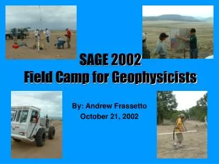
SAGE 2002Field Camp for Geophysicists By: Andrew Frassetto October 21, 2002
What is SAGE?: • Summer of Applied Geophysical Experience • Centered in Santa Fe, NM and run by Los Alamos National Lab and The University of California • Seven days of lectures on geophysical techniques (seismic, gravity, magnetic, electrical) • Seven days of field work (6 in the primary area, 1 at an archaeological site) • Four days of data analysis and interpretation
The Advantages: • One of the few opportunities for undergraduates to gain a skill in a wide variety of geophysical techniques • Exposure to numerous career paths via industry lectures (environmental, mining, petroleum) • An opportunity to practice geophysics in the Rio Grande Rift, an area of active extension in the Basin and Range Province
The Outcome: • Present a 12 minute talk on your topic: seismic reflection, seismic refraction, gravity, transient electromagnetics, magnetotellurics, the archeological site (GPR, refraction, magnetics, DC resistivity) or structural geology • Integrate results with other team members • Write a four-five page “expanded abstract” on your topic
Sediment Properties Determined with Magnetotellurics By: Andrew Frassetto University of South Carolina Presented on July 17, 2002
Outline: • Avoiding an “MT Stare”: An introduction to Magnetotellurics • Overview of the field area • Examples of MT Curves and 1-D Inversion Models • Description of the Geoelectric profile • My study: Determining sediment properties of shallow, low resistivity layer • Problems in determining sediment properties using Archie’s Law and Wyllie’s Equation • Summary of results and interpretations regarding porosity and seismic velocity • Implications of the sediment properties • Integrated results
The Basics of MT: • Low frequency, passive, deep imaging of lithosphere • Uses naturally occurring electric and magnetic fields (influenced by lightning strikes, solar storms, etc.) • Traditionally uses Ex and Ey, along with Hx, Hy, Hz (Titan-24 System did not measure Hz) (Jiracek et al., 1995)
MT at SAGE 2002: • On an MT curve, a positive slope indicates a resistive layer, while a negative slope shows increasing conductivity. The increasing period represents a lowering frequency at depth. (Jiracek et al., 1995) • SAGE 2002’s MT setup consisted of 41 separate • Data collection points spread at 100 m intervals over 4.1 km. The data was collected in two days.
MT at SAGE 2002: • MT sounding curves contain TE and TM components: TE assumes that Exis continuous across a conductive-resistive boundary. • A large separation of TE from TM on a curve represents a drastic change in the apparent resisitivity of layers. (Jiracek et al., 1995)
Field Area: MT/TEM Line N 8 km (Terraserver, 2002)
Field Area: Power Lines
Examples: App. Resistivity (ohm-m) Period (sec)
Examples: App. Resistivity (ohm-m) Period (sec)
Examples: App. Resistivity (ohm-m) Period (sec)
Examples: App. Resistivity (ohm-m) Period (sec)
Initial Observations: • From the 1-D Inversion model, four basic layers can be seen: • -a thin resistive surface layer • -a 150-650 m thick layer of low resistivity • -a 1000-1500 m thick layer of high conductivity • -the highly resistive basement at 2500-3500 m • The basement layer becomes shallower down the line, with the conductive layer becoming thinner • The subsequent 1-D Inversion stitch illustrates these layers fairly well
Geoelectric Profiles: Area of Focus Depth (m) Precambrian Basement: ~2.5-3.5 km depth Distance (km)
Geoelectric Profiles: Power Line Effect Depth (m) Distance (km)
Well Data: Data from a geochemical analysis were used to estimate the resistivity of water in this region using a Salinity-Porosity Nomogram. Thus, porosity can be calculated using Archie’s Law. Flora Barres Well (Longmire, 1985)
Calculations: The well data include temp (18.1 ˚C) and equivalent salinity (385 ppm). Plotting these on the Nomogram and connecting them with a best fit line yields ρw ≈ 14 ohm-m. (SAGE 2002 Notes)
Calculations - Porosity: Archie’s Law: ρr / ρw = aΦ-m …where a is the coefficient of saturation and m is the cementation factor. ρr was taken from the 1-D inversion model Values range from 8 ohm-m to 34 ohm-m, with most approximately 20 ohm-m. Humble Formula: a = 0.62, m = 2.15 …used in sand/sandstone environments and applicable to the SAGE 2002 field environment Archie’s Law cannot be applied to clay environments, as clay drastically increases the conductivity and renders porosity estimates useless.
Calculations - Seismic Velocity: Wyllie’s Equation: 1/v = Φ/vf + 1-Φ/vm …where vf is the velocity of the fluid and vm is the velocity of the matrix rock, in this case assumed to be granite. As such, vf = 1510 m/s and vm = 5375 m/s. (SAGE 2002 Notes)
Data: Calculated Results: Φ ≈ 29% vp = 3148.28 m/s Several data points were dropped due to power lines in center and clays near the end of MT line. (SAGE 2002 Notes)
Interpretations: Near river: more clay? Φ≈ 25-35%: potential aquifer Clay & possible increase in salinity?: poor aquifer
Conclusions: • Resistivities are a reasonable method to estimate the porosity of buried sediments or rocks. • Calculated values for porosity and sand are fairly consistent across the profile. • The values suggest a large amounts of loosely consolidated, non-lithified sediments (sand) to a depth of 660 m. • This region of basin has the potential to be an excellent freshwater aquifer.
Integrated Results: • Seismic Refraction – Velocity model for shallow layers, fault location • Seismic Reflection – Velocities, fault location • Gravity – Depth to Basement • TEM – Location of La Bajada fault, imaging of possible shallow resistive layers • MT – Depth to Basement, imaging of deeper conductive layer
TEM – Fault Location/Shallow Aquifer: La Bajada? (Ugarte and Larkin, 2002)
Seismic - Fault Location: Flag ~222 1800 m/s 1900 m/s Flag ~230 (Supak, 2002) (Parkman, 2002) 2000 m/s 2200 m/s
Gravity - Depth to Basement: (Khatun, 2002) • Gravity models show a basement depth that varies between 1.5 and 3.0 km at the basin end of the MT line. • SAGE 2002 gravity group believes the lowest model is correct
Depth to Basement Estimates: Gravity Estimates MT Estimate
Acknowledgements: • Quantec and Zonge Engineering for their equipment and expertise • Cochiti Pueblo for the privilege of working on their land • David Alumbaugh and George Jiracek for their guidance and expertise
References: Jiracek, G.R., Haak, V., Olsen, K.H., 1995, Practical magnetotellurics in a continental rift environment. In: K.H. Olsen (ed.), Continental Rifts: Evolution, Structure, and Tectonics, Developments in Geotectonics Vol. 25, Elsevier, Amsterdam, p. 103-128 Longmire, P., 1985, A Hydrogeochemical Study Along the Valley of the Santa Fe River, Santa Fe and Sandoval Counties, New Mexico. Ground Water and Hazardous Waste Bureau, Santa Fe, p. 01-35 Ward, S.H., 1990, Resistivity and induced polarization methods. In: Ward, S.H. (ed.), Geotechnical and environmental geophysics, Vol. 1, Society of Exploration Geophysicists, p. 147-189 SAGE 2002 Handbook