Download
1 / 59
600 likes | 878 Views
Chapter 10: Time and Global States. Introduction Clocks,events and process states Synchronizing physical clocks Logical time and logical clocks Global states Distributed debugging Summary. Introduction. Time is an important issue in DS Need to measure accurately

E N D
Chapter 10: Time and Global States • Introduction • Clocks,events and process states • Synchronizing physical clocks • Logical time and logical clocks • Global states • Distributed debugging • Summary
Introduction • Time is an important issue in DS • Need to measure accurately • E.g. auditing in e-commerce • Algorithms depending on • E.g. consistency, make • No universe physical clock • Newton’s opinion • Einstein’s Relativity Theory • People’s approaches • Approximately synchronize • Logical clocks • Capture causality between events
Chapter 10: Time and Global States • Introduction • Clocks,events and process states • Synchronizing physical clocks • Logical time and logical clocks • Global states • Distributed debugging • Summary
Model of a distributed system • £ • A collection of N processes pi, i = 1,2, .. N • si • The state of pi • E.g. variables • Actions of pi • Operations that transform pi’s state • Send or receive message between pj • e • Event: occurrence of a single action • i • occur before in pi , e.g. eie` • Total order of events in pi • history(pi ) = hi = <ei0, ei1, ei2, …>
Clocks • Clock in computer • A device that count oscillations occurring in a crystal at a definite frequency • hardware time: Hi(t) • Relative time • Software time: Ci(t) = Hi(t)+ • Timestamp of event • Clock skew and clock drift • Skew: the instantaneous difference between the readings of any two clocks • Drift: crystal oscillate at different rate • Can’t avoid clock drift • example
Coordinated Universal Time • Standard second • Atomic oscillator (International Atomic Time) • Drift rate: one part in 1013 • 9,192,631,770 periods of transition between the two hyperfine levels of the ground state of Cs133 • Since 1967 • Astronomical time • Rotation of earth on its axis and about the Sun • Skew between astronomical time and atomic time • Coordinated Universal Time (UTC) • Atomic time which is inserted a leap second occasionally to keep in step with astronomical time • Broadcast UTC to the World • E.g., by GPS or WWV
Chapter 10: Time and Global States • Introduction • Clocks,events and process states • Synchronizing physical clocks • Logical time and logical clocks • Global states • Distributed debugging • Summary
External & Internal synchronization • Ci: pi’s clock, I: an interval of real time • External synchronization • For a synchronization bound D > 0, and for a source S of UTC time, |S(t)-Ci(t)| < D, for i = 1, 2, … N and for all real times t in I • Clocks Ci are accurateto within the bound D • Internal synchronization • For a synchronization bound D > 0, |Ci(t)-Cj(t)| < Dfor i, j =1,2, … N, and for all real times t in I • Clocks Ciagreewithin the bound D • If accurate to within D, then agree within 2D
General synchronization measures • Correctness of a hardware clock H • A bounded drift rate , e.g. 106 seconds/second • (1 - )(t’ - t) <= H(t’) - H(t) <= ( 1 + )( t’ - t) • Correctness of a software clock • Monotonicity: t’ > t C(t’) > C(t) • Set clock back • Errors in the make • Change the clock rate • Clock failures • Crash failure: stop ticking • Arbitrary failure, e.g. Y2K bug
t t + min t +Ttrans t+max Synchronization in a synchronous system • Protocol • Sender: send M(t) • receiver: set time to t + Ttrans • Bounds are know in synchronous system • min < Ttrans < max • So, set Ttrans = (min+max) / 2 • Receiver clock = t + (min+max) / 2 • Clock skew • (max – min ) / 2
t + min t +Tround-min t t +Tround/2 t +Tround Cristian’s method of synchronizing clocks • Application circumstance • C/S Round-trip time is short compared with the required accuracy • Protocol • mr, mt, Tround • Estimated time: mt + Tround/2 • Accuracy analysis • If the minimum delay of a message transmission is min, then accuracy: (Tround/2 – min)
The Berkeley algorithms • Internal synchronization • Protocol • masterpollslaves’ clocks • master estimate slaves’ clocks by round-trip time • Similar to Christian’s algorithm • Average the slaves’ clock values • Cancel out the individual clock’s tendencies to run fast or slow • Send back to the client the amount that the client’s clock should adjust by • Positive or negative value • Avoid further uncertainty due to the message transmission time
Design aims of Network Time Protocol • External synchronization • enable clients across the Internet to be synchronized accurately to UTC • Reliability • can survive lengthy losses of connectivity • Redundant server & redundant path between servers • Scalability • Enable clients to resynchronize sufficientlyfrequently to offset the rates of drift found in most computers • Security • Protect against interference with the time service
Network Time Protocol • Architecture • Reconfigure as servers become unreachable • Synchronization measures • Multicast mode • Intend for use on a high speed LAN • Assuming a small delay • Low accuracy but efficient • Procedure-call mode • Similar to Christian’s • higher accuracy than multicast • Symmetric mode • The highest accuracy
Symmetric mode synchronization Assumming t, t’: actual transmission time of m, m’; o: actual B’s clock skew relative to A We have Ti-2 = Ti-3 + t + o , Ti = Ti-1 + t’ – o Then di = t + t’ = Ti-2 –Ti-3 + Ti – Ti-1 o = oi +(t’-t)/2 where oi= (Ti-2 –Ti-3 + Ti-1 –Ti ) /2 Estimated time:oi Accuracy analysis Due t, t’ >=0, then oi - di /2 <= o <= oi + di /2 di is the measure of the accuracy • Protocol, highest accuracy
Symmetric mode synchronization …continued • Implementation • NTP servers retain eight most recent pairs <oi,di> • The value oi of that corresponds to the minimum value di is chosen to estimate o • A NTP server exchange with several peers in addition to with parent • Peers with lower stratum numbers are favoured • Peer with the lowest synchronization dispersion are favoured
Chapter 10: Time and Global States • Introduction • Clocks,events and process states • Synchronizing physical clocks • Logical time and logical clocks • Global states • Distributed debugging • Summary
Happen-before relation • • HB1: If process pi: eie`, then ee` • HB2: For any message m, send(m) receive(m) • HB3: IF e, e`and e`` are events such that e e` and e` e``, then e e`` • Causal ordering or potential causal ordering • Example • a || e • Shortcomings • Not suitable to processes collaboration that does not involve messages transmission • Capture potential causal ordering
Logical Clock • Lamport timestamps algorithm • LC1: Li is incremented before each event is issueed at process pi : Li :=Li+1 • LC2: (a) When a process pi sends a message m, it piggybacks on m the value t = Li; (b) On receiving (m,t), a process Pj computes Lj := max(Lj, t) and then applies LC1 before timestamping the event receive(m) • e e` L(e) < L(e`) • L(e) < L(e`) e e` or e||e` • Example
Totally ordered logical clocks Assumming Ti: local timestamp of e that is an event occuring at pi Tj: local timestamp of e` that is an event occuring at pj Define the timestamps of e, e` are (Ti, i), (Tj, j) Define < (Ti, i) < (Tj, j) if Ti < Tj , or Ti = Tj and i < j • Useful in some applications
Vector Clocks • Algorithm • Each process pi keeps a vector clock Vi • VC1: Initially, Vi[j]=0, for i, j = 1,2…, N • VC2: Just before pi timestamps an event, it sets Vi[i] := Vi[i] +1 • VC3: pi includes the value t= Vi in every message it sends • VC4: When pi receives a timestamp t in a message, it sets Vi[j] :=max(Vi[j], t[j]), for j=1,2…,N • Compare vector timestamps • V = V` iff V[j] = V`[j] for j = 1,2…, N • V <= V` iff V[j] <= V`[j] for j = 1,2…, N • V < V` iff V <= V` and V <> V`
Vector Clocks …continued • Example • V(e) < V(e`) ee`, V(e) <> V(e`) e||e` • O(N) storage and message payload • N is unavoidable • Improvement • smaller data + reconstruct
Chapter 10: Time and Global States • Introduction • Clocks,events and process states • Synchronizing physical clocks • Logical time and logical clocks • Global states • Distributed debugging • Summary
Requirements of global states • Distributed garbage collection • Based on reference counting • Should include the state of communication channels • Distributed deadlock detection • Look for “waits-for” relationship • Distributed termination detection • Look for state in which all processes are passive • Distributed debugging • Need collect values of distributed variables at the same time
Global states and consistent cuts • The essential problem of Global states • Absence of global time • History of process pi:hi = <ei0, ei1, ei2 …> • Prefix of a process’s history: hik = <ei0, ei1… eik > • Global history of processes set £: H = h1h2 … hN • A global state:S = (s1, s2, … sN) • A cutof a system execution:C = <h1c1, h2c2… h3c3 > • Frontier of a cut:example • A cut C is consistent:For all events eC, fefC • <e10, e20> is inconsistent, <e12, e22> is consistent
Global states and consistent cuts … continued • A consistent global state:correspond to a consistent cut • The si corresponding to the cut C is that of pi immediately after the last event processed by pi in C – frontier of C • Execution of a distributed system:S0 S1 S2 … • A run:a total ordering of all the events in a global history that is consistent with eachlocal history’s ordering,i • Not all runs pass through consistent global state • A linearization (consistent) run: an ordering of the events in a global history that is consistent with this happened-before relationon H. • Pass only consistent global state • S` is reachable from a state S: there is a linearization that pass through S and then S`
Global state predicates, stability, safety and liveness • Global state predicates • A function that maps from the set of global states of processes in the system £ to {True, False} • Characteristics of global state predicates • Stability: once the system enters a state in which the predicate is True, it remains True in all future states reachable from that state • Useful in deadlock detecting, or termination detecting • Safety with respect to predicate : evaluates to False for all states S reachable from S0 • E.g., is a property of being deadlocked • Liveness with respect to predicate : for any linearization L starting in the state S0, Evaluates to True for some state SL reachable from S0 • E.g., is a property of reaching termination
The “snapshot” algorithm of Chandy and Lamport • Aim • Capture consistent global state of distributed system • Algorithm assumptions • Neither channels nor processes fail • unidirectional channels, FIFO message delivery • Complete connection among all processes • Any process may initiate a global snapshot at any time • process may continue execution and send and receive normal message while snapshot takes place
The “snapshot” algorithm • Idea • When one process record a state Si, make all other processes record states that have been caused by Si • Method • Incoming channels, outgoing channels • Process state + channel state • marker message • Marker sending rule: a process sends a marker after it has recorded its state, but before it send any other messages • Marker receiving rule: a process records its state if the state has changed since last recording, or record the states of the incoming channel • Algorithm
The “snapshot” algorithm - example • p1 trade p2 in widget which is 10$ per item • Initial state • p1 has sent 50$ to p2 to buy 5 widget, and p2 has received the order
Execution of the processes in the example • The final recorded state • P1:<$1000, 0>; p2:<$50,1995>;c1:<(five widgets)>;c2:<>
Characterising the observed state • The caught states are consistent • Examine two events ei, ej between pi and pj, such that eiej We want to prove: if ej occurred before pj recorded its state, then ei must have occurred before pi recorded its state The opposite of what we want to prove: pi recorded its state before ei occurred Proving: Because eiej, then there are messages m1, m2… at pj. Before these messages, there must be a marker saying pi has recorded its state These marker message let pj record state before ej So: the caught state is consistent
Characterising the observed state … continued • Construct reachability relationship • Reachability between the observed global state and the initial and final global states • Sys = e0, e1, … : linearization of the system as it executed • Find a permutation of Sys, Sys` = e0`, e1`, … such that all three states Sinit, Ssnap and Sfinal occur in Sys` • Sys` is also a linearization • Approach • Find pre-snap events / post-snap events according to a snap • figure
Chapter 10: Time and Global States • Introduction • Clocks,events and process states • Synchronizing physical clocks • Logical time and logical clocks • Global states • Distributed debugging • Summary
Distributed debug introduction • example • Safety condition of a distributed system: |xi-xj|<= • approach • A monitor • Collect states of other distributed processes • Apply a given global state predicate on the states • Possibly : there is a consistent global state s through which a linearization of H passes such that (s) is true • Definitely : for all linearizations L of H, there is a consistent global state set S through which L passes such that (S) is true
Observing consistent global states • Vector clock at each process • Timestamp each event occurring at each process • Each process send the timestamped event to the monitor • Find consistent global states by the monitor • Let S = (s1, s2, …, sN) • S is a global state drawn from the state messages that the monitor has received • S is a consistent global state if and only if V(si)[i]>=V(sj)[i] for i,j = 1,2,…, N • If one process’s state depends upon another, the global state also encompasses the state upon which it depends
Observing consistent global states … continued • Example of consistent global states and inconsistent global states • Two processes manage to maintain |x1-x2| <= 50 • When one process adjust the value of its variable largely, it informs the other process to adjust the other variable to than value either • The lattice of collected global states • Monitor construct the reachability lattice by the consistent global state identification algorithm • Find consistent global states • Establish the reachability relation between states • Sij is in level (i+j) • Show all the linearizations corresponding to a history
Evaluating possibly and definitely • Evaluating possibly • There is a downwards way in which there is a state evaluated to True by • Evaluating definitely • There is no downwards way in which there is not a state evaluated to True by • Example • If evaluates to True in the state at level 5, then definitely • If evaluates to false in the state at level 5, then possibly
Evaluating possibly and definitely in synchronous systems • Asynchronous systems • High time cost • To find consistent global state S = (s1, s2, …, sn), the monitor Should examine any two local states si and sj • Synchronous systems • |Ci(t)-Cj(t)| < D for i,j = 0, 1,…, N • Algorithm modification • The observed process sends vector time and physical time with the event to the monitor • Monitor find consistency state • V(si)[i]>=V(sj)[i] • si and sj should occurred at the same real time
Chapter 10: Time and Global States • Introduction • Clocks,events and process states • Synchronizing physical clocks • Logical time and logical clocks • Global states • Distributed debugging • Summary
Summary • Clock skew, clock drift • Synchronize physical clocks • Christian’s algorithm • Berkeley algorithm • Network Time Protocol • Logical time • Happen-before relation • Lamport timestamp algorithm • Vector clock
Summary …continued • Global states • Consistent cut, consistent state • Snapshot algorithm • Construct reachability relationship by snapshot • Global debugging • The monitor collects distributed events with vector timestamp • Construct reachability relationship • Examine possibly and definitely
m r m t p Time server,S Clock synchronization using a time server
1 2 2 3 3 3 Note: Arrows denote synchronization control, numbers denote strata. An example synchronization subnet in an NTP implementation
Server B T T i -2 i-1 Time m m' Time Server A T T i - 3 i Messages exchanged between a pair of NTP peers