Download
1 / 39
400 likes | 570 Views
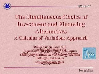
The Simultaneous Choice of Investment and Financing Alternatives A Calculus of Variations Approach. Robert W Grubbström Department of Production Economics Linköping Institute of Technology, Sweden rwg@ipe.liu.se. Robert W Grubbström Department of Production Economics

E N D
The Simultaneous Choice of Investment and Financing AlternativesA Calculus of Variations Approach Robert W Grubbström Department of Production Economics Linköping Institute of Technology, Sweden rwg@ipe.liu.se Robert W Grubbström Department of Production Economics Linköping Institute of Technology, Sweden rwg@ipe.liu.se - An Invited Lecture for The A.M.A.S.E.S. XXIV Conveigna Padenghe sul Garda September 6-9, 2000 - An Invited Lecture for The A.M.A.S.E.S. XXIV Conveigna Padenghe sul Garda September 6-9, 2000 The Simultaneous Choice of Investment and Financing Alternatives A Calculus of Variations Approach
Orlicky To Lorenzo Peccati and Marco Li Calzi : Many thanks for giving me and my wife Anne-Marie the opportunity to come to Padenghe! Molte grazie!!
Backgroundmotives Backgroundmotives
2 Reasons for thinking in Cash terms The Cash Flow (and what you can do with it) is the ultimate consequence of all economic activities The Cash Flow is the nearest you can get to finding a physical measure of economic activities “A principle for determining the correct capital costs of work-in-progress and inventory”, International Journal of Production Research, 18, 1980, 259-271
Staircase function Staircase function
The Product Structure, the Gozinto Graph and the Input Matrix The Product Structure, the Gozinto Graph and the Input Matrix
The Input Matrix and its Leontief Inverse Leontief Inverse Input Matrix The Input Matrix and its Leontief Inverse
Adding the Lead Time Matrix and Creating the Generalised Input Matrix Lead Time Matrix Generalised Input Matrix Adding the Lead Time Matrix and Creating the Generalised Input Matrix
Leontief Inverse and Generalised Leontief Inverse Generalised Leontief Inverse ~ Leontief Inverse and Generalised Leontief Inverse Leontief Inverse
Inventory and Backlog Relationships Inventory and Backlog Relationships
Conclusion Conclusion • When studying complex multi-level, multistage production-inventory systems, there is an essential need to be aware of what the basic objective should be interpreted as. • The discussion to follow has the purpose to justify the use of the Net Present Value as the sole objective.
References For references please consult: http://ipe.liu.se/rwg/mrp_publ.htm Recent survey: Grubbström, R. W., Tang, O., An Overview of Input-Output Analysis Applied to Production-Inventory Systems, Economic Systems Research, Vol. 12, No 1, 2000, pp. 3-26 Recent thesis: Tang, O., Planning and Replanning within the Material Requirements Planning Environment – a Transform Approach, PROFIL 16, Production-Economic Research in Linköping, Linköping 2000 References
Currentproblem Currentproblem
General Problem General Problem The problem considered is to choose from a finite set of inter-related investment and financing alternatives and also levels of consumption/work over time to maximise a utility functional. Each investment and financing option is characterised by its cash flow over time. An inter-temporal budget requirement operates continuously. Application of the Calculus of Variations leads to consideration of the Euler-Lagrange equations combined with Kuhn-Tucker conditions. It is shown that the solution (also when there are logical dependencies present) requires the maximisation of a Generalised Net Present Value measure in which the discount factor is formed from an integral of a Lagrangean multiplier function.
Calculus of Variations Joseph-Louis Lagrange 1736-1813 Leonhard Euler 1707-1783 Calculus of Variations Around 1755 Developed by Joseph-Louis Lagrange (Giuseppe Lodovico Lagrangia), 1736-1813, (then only 19 years old). Name suggested by Leonhard Euler, 1707-1783. Original Problems *Find the maximum area enclosed by a curve of given length. *The Brachistochrone problem: To specify a path between two given points in space, such that a particle released at a given velocity will slide from the upper to the lower point under gravity in the minimum time.
Basic Methodology A functional (an integral) is to be optimised. This is the objective function. The problem is to find the path x(t). The integrand H is called the Hamiltonian. The necessary local optimisation conditions read: A functional (an integral) is to be optimised. This is the objective function. The problem is to find the path x(t). The integrand H is called the Hamiltonian. The necessary local optimisation conditions read: These are the Euler-Lagrange Equations. In the following these conditions will be extended slightly with the use of the ”modern” Kuhn-Tucker conditions in order to take care of non-negativity requirements. Basic Methodology A functional (an integral) is to be optimised. This is the objective function.
Discrete time comparison A non-rigorous comparison with a Lagrangean discrete optimisation is the following. Let and optimise by a suitable choice of the , where . A non-rigorous comparison with a Lagrangean discrete optimisation is the following. Let and optimise by a suitable choice of the , where . Let be Lagrangean multipliers. The Lagrangean is written: Multiplier Discrete time comparison
Discrete time comparison II Necessary Lagrangean conditions: Necessary Lagrangean conditions: Eliminating the leads to Discrete time comparison II
Discrete time comparison III Take the following limits and while keeping . Then: Discrete time comparison III
Utility functional Utility functional
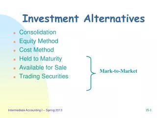
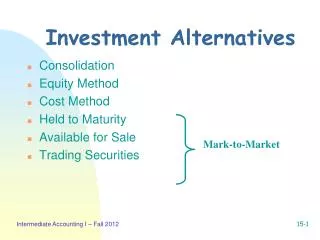
Types of Cash Flows Types of Cash Flows • Money earned from work and money paid for consumption. • Investment projects or loans with a fixed payment scheme. These cash flows can be accepted partially or completely. • Variable loans or short-term investment alternatives which can be varied over time. An interest rate, possibly time varying, is attached to each such cash flow. • Interest payments attached to each variable loan or short-term investment.
Andrew Vazsonyi The Budget Box The Budget Box
Variable Loan + Interest Variable Loan + Interest
Budget Constraint Budget Constraint
Other Constraints Decision variables for fixed payment schemes Possible logical constraints for investments etc. Repayment constraints for loans Other Constraints
Lagrangean function Multiplier Multiplier Multiplier Multiplier Lagrangean function
Lagrangean function Hamiltonian Lagrangean function
Euler-Lagrange Conditions I Euler-Lagrange Conditions I
Euler-Lagrange Conditions II Euler-Lagrange Conditions II Remember, for variable loans/short-term investments: Then:
Consequences I So, whenever , we have the important solution: Or, when : The normalised Lagrangean multiplier integral is therefore the discount factor! Consequences I
Kuhn-Tucker Conditions Net Present Value NPV except for Kuhn-Tucker Conditions
Consequences II If then and then . If then, since , we have . Consequences II Disregarding (temporarily) logical constraints: lead to:
Consequences III For instance, when there is both consumption and work, then . Then, if marginal momentary utility decreases with x (becomes more negative with y) and time preferences (the t in u(x,y,t)) are disregarded, we must have a greater x for a greater t, and a lower y for a greater t. Consequences III Marginal utilities and discount factor: Mathematical justification of Bertrand Russel’s statement: “Forethought, which involves doing unpleasant things now, for the sake of pleasant things in the future, is one of the most essential marks of the development of man.” with equalities whenever x > 0 or y > 0.
Consequences IV Assume, for instance, a separable case: which means that must be proportional to . Consequences IV If there is both consumption and work, which keep at the same levels over time, x=const and y=const, then the time preference must follow the discount factor. Then:
Example 10000 7945 Utility function Loan at 20 % p.a. Short-term investment at 10% p.a. Investment initial outlay -10000, inflow +2000 p.a. 2815 2240 -410 20.0 14.26 17.30 3.06 Example
Conclusions Conclusions • The Net Present Value, appropriately defined, is a superior measure of the benefit of a cash flow. • The Calculus of Variations appears to be tailor made for analysing investment and financing alternatives.
Main references Main references Grubbström, R. W., Ashcroft, S. H., Application of the Calculus of Variations to Financing Alternatives, Omega, Vol. 19, No 4, 1991, pp. 305-316 Grubbström, R.W., Jiang, Y., Application of the Calculus of Variations to Economic Decisions: A survey of some economic problem areas, Modelling Simulation and Control, C, Vol. 28, No 2, 1991, pp. 33-44
There is more to life than making money… But, I do think it is important for a person to have something to do, when he’s not drinking or making love ...
Orlicky Thank you for your kind attention!