Download
1 / 36
720 likes | 2.78k Views
Chapter 4 Excess Carriers in Semiconductors. 4.1 Optical Absorption 4.2 Luminescence 4.3 Carrier Lifetime and Photoconductivity 4.4 Diffusion of Carriers. 4.1 Optical Absorption(1).

E N D
Chapter 4Excess Carriers in Semiconductors 4.1 Optical Absorption 4.2 Luminescence 4.3 Carrier Lifetime and Photoconductivity 4.4 Diffusion of Carriers
4.1 Optical Absorption(1) • hv > Eg : Optical absorption EHP The excited electron gives up energy to the lattice by scattering events The electron recombines with a hole in the valence band. • hv < Eg : Optical absorption Transparent in certain wavelength ranges. Ex) NaCl : Eg 3 eV : Allow infrared and the entire visible spectrum to be transmitted.
4.1 Optical Absorption(4) • Si absorbs not only band gap light (~1um) but also shorter wavelengths, including those in the visible part of the spectrum.
4.2 Luminescence • Luminescence : Light emission (The radiation resulting from the recombination of the excited carriers) - Photoluminescence : If carriers are excited by photon absorption. - Cathodoluminescence : If the excited carriers are created by high-energy electrom bombardment of the material. - Electroluminescence : If the excitation occurs by the introduction of current into the sample.
4.2.1 Photoluminescence • Light Absorption → EHP excitation → the recombination of EHPs Light emission • Direct recombination : Fast process → Fluorescence - The mean lifetime of the EHP < 10-8s - The emission of photons stops within approximately 10-8s after the excitation is turned off. • Emission continues for periods up to seconds or minutes after the excitation is removed → Phosphorescence
4.2.1 Photoluminescence • An incoming photon with hv1 > Eg is absorbed, creating an EHP. • The excited electron gives up energy to the lattice by scattering until it nears the bottom of the conduction band. • The electron is trapped by the impurity level Et • and remains trapped until it can be thermally reexcited to the conduction band. • Finally direct recombination occurs as the electron falls to an empty state in the valence band, giving off a photon (hv2) of approximately the band gap energy.
4.2.1 Photoluminescence • Ex 4-1> • A 0.46um-thick sample of GaAs is illuminated with monochromatic light of hv=2V. The absorption coefficient α is 5×104 cm-1. The power incident on the sample is 10mW. • Find the total energy absorbed by the sample per second (J/s). • SOL>
4.2.1Photoluminescence (b) Find the rate of excess thermal energy given up by the electrons to the lattice before recombination (J/s). SOL> (c) Find the number of photons per second given off from recombination events, assuming perfect quantum efficiency. SOL>
CRT Cathode Ray Tube 4.2.2 Cathodoluminescence • Emission of excited electron on cathode → Acceleration to anode → Atom excitation in phosphor → Light emission by recombination 4.2.3 Electroluminescence • LED - Recombination between minority carrier and majority → Light emission
Thermal generation Number of electrons remaining at t 4.3 Carrier Lifetime and Photoconductivity • Photoconductivity - If the excess carriers arise from optical luminescence, the resulting increase in conductivity is called Photoconductivity 4.3.1 Direct Recombination of Electrons and Holes (1) • Net rate of change in the conduction band electron concentration } }
4.3.1 Direct Recombination of Electrons and Holes (2) • Let us assume the excess electron-hole population is created at t=0 and the initial excess electron and hole concentration Δn and Δp are equal. Then as the electrons and holes recombine in pairs, the instantaneous concentrations of excess carriers δn(t) and δp(t) are also equal. • If the excess carrier concentration are small, we can neglect the δn2 term and if the material is p-type (p0>>n0), • Excess electrons in a p-type semiconductor recombine with a decay constant τn=(αnp0)-1, called the recombination lifetime.
4.3.1 Direct Recombination of Electrons and Holes (3) Ex 4-2> GaAs. NA = 1015 cm-3, n i = 106 cm-3, n0 = ni2/p0 = 10-3 cm-3 If 1014 EHP cm-3 are created at t=0, n = p = 10-8 s. General recombination life-time => Minority carrier decay is more important
4.3.2 Indirect Recombination; Trapping (1) • The vast majority of the recombination events in indirect materials occur via recombination levels within the band gap, and the resulting energy loss by recombining electrons is usually given up to the lattice a heat rather than by the emission of photons. • When a carrier is trapped temporarily at a center and then is reexcited without recombination taking place. → Temporary trapping. → Recombination delay
Photoconductivity decay Estimation of Recombintion or trapping effect 4.3.2 Indirect Recombination; Trapping (3) • The conductivity of the sample during the decay (t) = q[n(t)n+p(t)p]
} New steady state value 4.3.3 Steady State Carrier Generation; Quasi-Fermi Levels (1) • Thermal equilibrium - Thermal generation of EHPs at a rate g(T)=gi • If a steady light is shone on the sample, For steady state recombination and no trapping, n=p. Neglecting the n2 term for low-level excitation,
4.3.3 Steady State Carrier Generation; Quasi-Fermi Levels (2) Steady state excess carrier concentration Minority carrier concentration (equilibrium) Steady state (steady state) * Equilibrium : When excess carriers are present :
4.3.3 Steady State Carrier Generation; Quasi-Fermi Levels (3) • Equilibrium : When excess carriers are present : : Quasi-Fermi Level Ex 4-4> steady state, * The excitation cause a large percentage change in minority carrier hole concentration and a relatively small change in the electron concentration
4.4 Diffusion of Carriers 4.4.1 Diffusion Processes (1)
4.4.1 Diffusion Processes (2) • Carriers in a semiconductor diffuse in a carrier gradient by random thermal motion and scattering from the lattice and impurities
: mean free path : mean free time 4.4.1 Diffusion Processes (3) •A rate of electron flow in the +x-direction per unit area •Difference in electron concentration The net motion of electrons due to diffusion is in the direction of decreasing electron concentration The resulting currents are in opposite directions
é ù dV(x) d E 1 dE e = = = i i ( x) - - ê ú dx dx dx ( -q) q ë û 4.4.2 Diffusion and Drift of Carriers; Built-in Fields (2) •Electron Potential Electrons drift “downhill” in the field
Dn Dp n p (cm2/s) (cm2/s) (cm2/V-s) (cm2/V-s) Ge 100 50 3900 1900 Si 35 12.5 1350 480 GaAs 220 10 8500 400 4.4.2 Diffusion and Drift of Carriers; Built-in Fields (3) •At equilibrium : no net current •The equilibrium Fermi level does not vary with x. Einstein relation Table 4-1 Diffusion coefficient and mobility of electrons and holes for intrinsic semiconductors at 300K
4.4.3 Diffusion and Recombination; The Continuity Equation(1) Rate of hole buildup Increase of hole concentration in δxA per unit time - Recombination rate = : Continuity equation for holes Continuity equation for electrons
4.4.3 Diffusion and Recombination; The Continuity Equation(2) •When the current is carried strictly by diffusion (negligible drift), Diffusion eq. for electrons Diffusion eq. for holes
4.4.4 Steady State Carrier Injection; Diffusion Length(1) •Steady state •Diffusion equation in the steady state : electron diffusion length : hole diffusion length •x=0 , steady state hole injection (p) p(x=0) = p LP : Distance at which the excess hole distribution is reduced to 1/e of its value at the point of injection
4.4.4 Steady State Carrier Injection; Diffusion Length(2) •Lp : Average distance a hole diffuses before recombining. Find Lp! •Probability that a hole injected at x=0 survives to x without recombination •Probability that hole at x will recombine in the subsequent interval dx •Total probability that a hole injected at x=0 will recombine in a given dx is the product of the two probabilities •Average distance a hole diffuses The diffusion current at any x is just proportional to the excess concentration δp at that position
Drift velocity Mobility 4.4.5 The Haynes-Shockley Experiment (1) •n-type : n0 >> p0 n : negligible p : significant •As the pulse drifts in the E-field it also spreads out by diffusion. By measuring the spread in the pulse, we can calculate Dp. → Gaussian Distribution
•Choosing the point Δx/2, at which is down by 4.4.5 The Haynes-Shockley Experiment (2) •Peak value of the pulse at any time (at x=0)
4.4.5 The Haynes-Shockley Experiment (3) •Since x cannot be measured directly, we measure t.
4.4.5 The Haynes-Shockley Experiment (4) Ex 4-6> Haynes-Shockley Experiment n-type Ge, length of the sample : 0.95cm, E0=2V A pulse arrives at point (2) 0.25ms after injection at (1) The width of the pulse t = 117 s p, Dp?
4.4.6 Gradients in the Quasi-Fermi Levels (1) •Equilibrium •Nonequilibrium excess carrier EF Fp or Fn •If we take the general case of nonequilibrium electron concentration with drift and diffusion. Thus, the processes of the electron drift and diffusion are summed up by the spatial variation of the quasi-Fermi level.
4.4.6 Gradients in the Quasi-Fermi Levels (2) •In the form of a modified Ohm’s law, Therefore, any drift, diffusion, or combination of the two in semiconductor results in currents proportional to the gradients of the two quasi-Fermi levels. * Equilibrium n0p0 = ni2 Steady-state np = ?