Isoparametric elements and solution techniques
Isoparametric elements and solution techniques. = ½ d 1-2 T k 1-2 d 1-2 +. + ½ d 2-4 T k 2-4 d 2-4 +….= = ½ D T KD. R=KD. gauss elimination computation time: (n order of K, b bandwith). recall: gauss elimination. rotations. isoparametric elements.

Isoparametric elements and solution techniques
E N D
Presentation Transcript
= ½ d1-2Tk1-2d1-2 + + ½ d2-4Tk2-4d2-4 +….= = ½ DTKD
R=KD • gauss elimination • computation time: (n order of K, b bandwith)
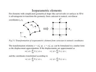
isoparametric elements isoparametric: same shape functions for both displacements and coordinates
computation of B • x = du / dX • but u=u(, ), v=v (, )
no strain at the Gauss points so no associated strain energy
The FE would have no resistance to loads that would activate these modes Global K singular Usually such modes superposed to ‘right’ modes
the locations of greatest accuracy are the same Gauss points that were used for integration of the stiffness matrix
Rayleigh-Ritz method Guess a displacement set that is compatible and satisfies the boundary conditions
define the strain energy as function of displacement set • define the work done by external loads • write the total energy as function of the displacement set • minimize the total energy as function of the displacement and find • simulataneous equations that are solved to find displacements
= (d) d / d d1 = 0 d / d d2 = 0 d / d d3 = 0 d / d d4 = 0 …… d / d dn = 0
patch tests • only for those who develops FE
divide the FEmodel in more parts • create a FE model of each substructure • Assemble the reduced equations KD=R • Solve equations
Constraints CD – Q =0 C is a mxn matrix m is the number of constraints n is the number of d.o.f. How to impose constraints on KD=R
way 1 – Lagrange multipliers =[1 2 …. m]T T [CD-Q]=0 = 1/2DTKD – DTR + T [CD-Q]
remember dAD / dD = AT dDTA/ dD = A
½tT t = ½ [(CD-Q)T(CD-Q)]= = ½ [(CD-Q)T(CD- Q)]= = ½ [(CD-Q)TCD- (CD-Q)T Q)]= = ½ [(DTCTCD-QTCD-DTCTQ +QTQ)]= ½[·]; d(½[·])/dD= =½[2(CTC)-(QTC)T- CTQ]= =½[2(CTC)-(C)TQ- CTQ]= =½[2(CTC)-CT Q- CTQ]=
=½[2(CTC)-CT Q- CTQ]= = CTC-CT Q (= T)