Database Design
Database Design. Database. A database is a collection of information that is organized so that it can easily be accessed, managed, and updated Databases typically contain aggregations of data records or files , such as chemical analysis, experiments, investigators, and sample

Database Design
E N D
Presentation Transcript
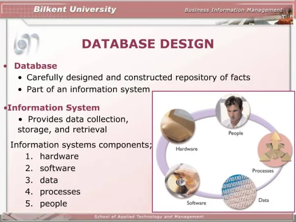
Database • A database is a collection of information that is organized so that it can easily be accessed, managed, and updated • Databases typically contain aggregations of data records or files, such as chemical analysis, experiments, investigators, and sample • Typically, a database manager provides users the capabilities of controlling read/write access, specifying report generation, and analyzing usage
Database structure • Databases are organized by columns, records, and tables • A column is a single piece of information; a record is one complete set of columns (shown in a row); and a table is a collection of records • For example, a telephone book is analogous to a table. It contains a list of records, each of which consists of three fields: • name, address, and telephone number • To access information from a database, you need a Database Management System (DBMS), e.g., MS Access • This is a collection of programs that enables you to enter, organize, and select data in a database
Relational Database • A relational database is a collection of data items organized as a set of tables from which data can be accessed or reassembled in many different ways without having to reorganize the database tables • The relational model specifies that the rows of a table have no specific order and that the rows, in turn, impose no order on the attributes • Applications access data by specifying queries, which use operations such as selectto identify rows, project to identify attributes, and join to combine relations (tables) • Relations (Tables) can be modified using the insert, delete, and update operators.
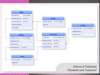
... • A relational database is a set of tables containing data organized into predefined categories • Each table (which is sometimes called a relation) contains one or more data categories in columns (fields) • Each row contains a unique instance of data for the categories defined by the columns • For example, a typical Investigator database would include a table (Investigator) that describes an investigator with columns (fields) for name, address, phone number, affiliation, degree, etc. • Another table (e.g., Sample) would describe fields such as sample_id, number, type, lithology, date taken, etc.
Relational Model • Relational model was developed by E.F. Codd in 1970, and is the basis for all RDBs • It uses the set theory for database modeling, based on relational algebra (RA) which is used to manipulate objects in a RDB • It involves the required information that may not appear in the UML diagram but is needed for the database • SQL is a declarative language, used to manipulate RDBs applying relational algebra
Table (Relation) • A table is defined as a set of rows that have the same attributes (fields under columns) • That is, a table is organized into rows and columns • A row usually represents one object and information (record) about that object • Objects are typically physical objects or concepts
View of the Database • A user of the database could obtain a view of the database that fitted the user's needs • For example, a head of a Geological Survey might like a view or report on: • all geological quadrangle maps that were completed by a certain date • A geologist in the same survey could, from the same tables, obtain a report on: • collected samples which need chemical analysis
… • In addition to being relatively easy to create and access, a relational database has the important advantage of being easy to extend • After the original database creation, a new data category (e.g., table) can be added without requiring that all existing applications be modified
Create a model of the real world • Design of a database involves modeling the domain (here it means universe of discourse) • Model: simplified abstraction of the real world • The database should contain information needed by the people who use it • UML (Unified Modeling Language) is perhaps the best modeling tool, along with ERD (entity relationship diagram) • We will model our database in MySQL Workbench or Microsoft Access
UML Class Diagram • UML class diagrams are used to define classes (equivalent to entity in ER diagrams) • Each class represents a type for all physical and conceptual things or an event • For example, Ocean, Aquifer, Mineral, Folding • First step: Define the class in English, e.g., • Aquifer: “A rock unit that can store and transmit economically significant amount of water” • Each class (singular form) has several attributes, which define the relevant descriptive (natural) properties or characteristics (those other than ID, keys) of each member of the class. Aquifer name type porosity thickness transmissivity hydraulicCond
Relation (Table) Schema • The UML class is translated into a relation schema identified by the class name (Aquifer) with all the attributes of the class, e.g.,: • Aquifer schema: Assignment rule: Associates each attribute to a set of valid values (i.e., defines the domain)
Data Integrity • When creating a relational database, we define the domainof possible values in a data column (i.e., for each attribute) and further constraints that may apply to that data value • This is done for data integrity so that invalid values will not be entered into the database • e.g., DATETIME, STRING, CHAR, INT • Domain: Set of valid values that can be assigned to an attribute • This can be done by assigning character length, data type, format, e.g., of email and URL address, zip codes, state names, etc. • Many of these should be handled with the user interface (in forms to collect user data), and enumerated lists
Constraints • Constraints allow further restriction of the domain of an attribute. • You can place constraints to limit the type of data that is stored in a table • For example, a constraint can restrict a given integer attribute to values between 1 and 5
Unique constraint • A UNIQUE constraint ensures that all values in a column are distinct (i.e., not duplicated) CREATE TABLE Customer (customer_id integer UNIQUE, last_name VARCHAR(100), first_name VARCHAR(100)); In this example, the customer_id column has a unique constraint, and cannot include duplicate values
Unique Constraint … • If the previous table already has a customer_id with a value of ‘3’, executing the following SQL statement, will result in an error because '3' already exists in the ID column: INSERT INTO Customer values ('3','Jones','Kaila'); • Trying to insert another row with that value violates the UNIQUE constraint
Default Constraint • A DEFAULT constraint provides a default value for a column when the INSERT INTO statement does not provide a specific value CREATE TABLE Student ( student_id INTEGER UNIQUE NOT NULL, last_name VARCHAR (100), first_name VARCHAR (100), score INTEGER DEFAULT 75);
Default value … INSERT INTO Student (student_id, last_name, first_name) VALUES ('1','James','Alex'); • The populated Student table will look like the following after execution: • Even though we didn't specify a value for the “score" column in the INSERT INTO statement, it does get assigned the default value of 75 since we had already set 75 as the default value for this column
Check Constraint • A CHECK constraint ensures that all values in a column satisfy certain conditions. Once defined, the database will only insert a new row or update an existing row if the new value satisfies the CHECK constraint • The CHECK constraint is used to ensure data quality • For example, in the following CREATE TABLE statement, CREATE TABLE Customer (customer_id integer CHECK (customer_id > 0), last_namevarchar (30), first_namevarchar(30)); • Column “customer_id" has a constraint -- its value must only include integers greater than 0. So, attempting to execute the following statement, will result in an error because the values for ID must be greater than 0 INSERT INTO Customer values ('-5','Smith','Lynn'); // leads to error
Set notation A schema is represented by a set notation Aquifer= {name, type, porosity, permeability, …} • Order of the attributes does not matter • Attributes cannot be duplicated • Rules can define domains for each element of the set • Can also limit the domain of an attribute to a specific range of values • We can define subset of the set (e.g., views) • All can be manipulated with set operators (e.g., union, to combine two relations or tables)
Relation =Table • The structure of each relation schema defines a table • Use SQL syntax to create a table: CREATE TABLE Aquifer ( id INT NOT NULL, name VARCHAR(20) NOT NULL, type VARCHAR(30) NOT NULL, porosity VARCHAR (10) NULL, permeability VARCHAR (20) NULL PRIMARY KEY (‘id’)); Variable-length character string i.e., value must be provided (not optional)
Rows represent individual objects • While each UML class become a table, values for each individual object, i.e., real world member of a class become a row in the table • Each row is a record • Each row (tuple) is a function that assigns a constant value to each attribute of the schema • e.g., function of name, type, porosity, … INSERT INTO Aquifer (name, type, porosity, location) VALUES (‘Floridan’, ‘confined’, ‘’, ‘Florida’); This (green) part can be omitted if values entered in order
Rows can be updated After a table is populated, the values in each row can change using the update clause: UPDATE Aquifer SET name = ‘High Plains’ WHERE name= ‘Ogallala’;
Table is a set of rows • Table is a set of rows with common attributes • Each row is unique • Rows are unordered • Can get a subset of the rows with SQL • Can use union, intersection, or difference of the rows in two or more tables if they have the same schema
Primary Key (PK) • It is a set of attributes that guarantee the uniqueness of each row in a table • A primary key can consist of one or more fields in a table. When multiple fields are used as a primary key, they are called a composite key • (used in junction tables in 1:m relationships) • Each primary key value must be unique within the table Table CUSTOMER CREATE TABLE Customer ( customer_id integer PRIMARY KEY, last_name VARCHAR (100), first_name VARCHAR(100) );
Foreign Key (FK) • A foreign key is a field (or fields) that points to (i.e., references) the primary key of another table • The purpose of the foreign key is to ensure referential integrity of the data • Meaning: only values that are supposed to appear in the database are permitted CREATE TABLE Analysis ( analysis_id integer primary key, analysisDatedatetime, analyzer_id integer references Analyzer (analyzer_id)); // The analyzer_id in the Analysis table references the analyzer_id attribute of the Analyzer table. Each analyzer may analyze many analyses Each analysis is done by only one analyzer Analysis Analyzer PK analysis_id analyzer_id analysisDate … analyzer_id … PK FK
Index • An index provides capability for quick access to data • That is, it speeds up the retrieval of data • Creating the proper index can drastically increase the performance of an application • A database index is used in much the same way a reader uses a book index • When a database has no index to use for searching, the result is similar to the reader who looks at every page in a book to find a word (or looks in a library to find a book): • The database engine needs to visit every row in a table. • In database terminology this is called a table scan
Index… • Index be created on any combination of attributes on a table CREATE TABLE Subscriber (subscriber_id INT PRIMARY KEY,email_address VARCHAR(255),first_name VARCHAR(255),last_name VARCHAR(255)); • If you want to quickly find an email address, create an index on the email_address field:CREATE INDEX Subscriber_email ON Subscriber (email_address); • Note: Subscriber_email is the name of the index • This SQL statement allows us to quickly find an email address:SELECT first_name, last_name FROM Subscriber WHERE email_address='email@domain.com'; Subscriber subscriber_id email_address first_namelast_name PK Index
Creating an Index Employee CREATE TABLE Employee ( employee_id INT PK, emp_name VARCHAR (200), ); • When you first create a new table, there is no index created by default • Use the following statement to create an index for this table CREATE INDEX employee_name ON Employee (emp_name); employee_name is an arbitrary name, given to the index for easy access (it may be different from the attribute in the table) employee_id emp_name PK Index
1 0..* UML Associations Aquifer Well PK aquifer_id aquifer_name aquifer_type … well_idlocation depth aquifer_id … PK FK • Indicate the way tables are functionally related to each other(in ER it is called relationships) • Relationship between Well class and Aquifer class • The association will help us to find out which wells penetrate a given aquifer • We start by describing the association in natural language, focusing on how many individuals of one class participate, or are connected, to a single individual of the other class, and vice versa (i.e., in both directions) • Each aquifer is drilled by zero or more wells (0..*) • Each well drills into only one aquifer • These statements help to identify the multiplicity(or cardinalityin ER) of the association
Multiplicity or cardinality Each aquifer is drilled by zero or more wells (0..*) Is drilled by 0..* 1..1 drills into Aquifer Well well_id number location type isCased Depth aquifer_id aquifer_id name type porosity thickness transmissivity hydraulicCond aquifer one and only one (1..1) drills into each well The maximum multiplicity indicates that this is a one-to-many association NOTE: The association name is the verb that describes the action (e.g., ‘drills into’ or ‘is drilled by’)
The Foreign Key represents UML association • For the 1..* association, we store the PK attribute of the ‘one’ side (Aquifer) into the table of the many (Well) • See previous slide • The copied PK becomes an FK (foreign key) • The ‘one’ side of the association is the ‘parent’ and the ‘many’ side is the ‘child’ of the association • Note: cannot have a child (well) without the parent (Aquifer) • Parent provides the PK; child receives it as FK • In other words: ‘one parent PK; many children FK! • The FK in the ‘many’ side may be used as the PK, for example, if we want to uniquely associate a well to an aquifer, or, the table may have its own PK in addition to the FK!
Aquifer-Well Association 1..1 Parent child 0..* Aquifer Well well_id number location type isCased Depth aquifer_id aquifer_id name type porosity thickness transmissivity hydraulicCond 1..1 0..* Parent child
Referential Integrity • The FK added to the child table must have the same type and size as the PK in the parent table ALTER TABLE Well ADD CONTRAINT well_id PRIMARY KEY (number, location); // primary key is a composite key // let’s decide that the FK in the Well table is called wellFK // Define the FK; say where they are found as PK ADD CONSTRAINT wellFKFOREIGN KEY (aquifer_name, aquifer_location) REFERENCES Aquifer (name, location); • The FK constraints ensures that each well contains a valid aquifer name and location • This maintains the referential integrity of the database
Updated Well Table • Aquifer data • Well data • NOTE: • Some aquifers (e.g., Floridan) are repeated in the Well table • The Aquifer data are copied in the foreign key fields (i.e., the first two columns)
One-to-One Association Entity Entity 1:1 • There are rare cases where the relationship between two types of data is one-to-one (1..1) • Each item has a relationship to only one item of the other type • e.g., the state name (Georgia) and its abbreviation (GA) • The mineral name and its formula (if it is constant) • Fold_Limb and Fold (composition) • Brain and Body (composition; will be covered later) • In such a case, the two items are included as two columns in one table • However, if in the future the relationship changes or the table is too big, it is better to break them into two tables
One-to-Many Association Entity Entity 1:M • One row in one table links to many rows in another, e.g.: • One geologist having published many papers • One person taking several samples • One sample having multiple analyses • The two entities in the one-to-many relationship (1..*) must be split into two tables • Note: A many-to-many (M:M) relationship is broken into two 1..* relationships (see next slides)
Many-to-many Association Entity Entity M:M • The relationship between some tables may be many-to-many, when: • many rows in one table are linked to many rows in another table • Each geologist may study many samples • Each sample may be studied by many geologists studies Sample Geologist 0..* 0..* isStudiedBy sample_id number type geologist_id name specialty affiliation
M:M … • Since the two tables cannot be children of each other, we cannot show m:m associations directly • There is no place to put the FK • So, we create a junction (association, intermediary) table, where the foreign keys of the two tables go (in addition to other attributes, if any). This creates two 1:M associations • Connect the junction table with a dotted line to association line studies 1..1 0..* 0..* 1..1 Study Sample samplePK number type studyPK type result geolPKsamplePK Geologist geolPK name specialty affiliation FKs The Study table has many records of one geologist and many records of one sample!
Generalization/Specialization • In many cases the attributes of a class (e.g., Fault) may be inherited by several subclasses (NormalFault, ReverseFault, StrikeSlipFault) • While the superclass generalizes the subclasses by providing the common attributes, the subclasses are said to specialize the superclass by adding additional unique attributes and behavior • The hollow arrow represents the ‘is-a’ relationship Fault 1..1 0..1 0..1 NormalFault ReverseFault Sibilings • Each normalFault or reverseFault is-a fault (one-to-one taxonomic relationship)
Generalization/Specialization … • In this case the relationships are one-to-one • The primary key of the superclass will become the foreign key in the subclass which will also be the primary key for the subclass Fault table 1..1 ReverseFault table NormalFault table 0..1 0..1
Aggregation • A system is an aggregate of several components (parts) • The components can exist on their own without being part of the system, e.g., a shear zone may be aggregated from a set of foliation, lineation, mylonite, cataclasite, vein, etc. • These can exist on their own even after the fault dies. • Tires, wheels, batteries, and engine of a car are other examples • Human head, hand, and other parts are NOT examples of aggregation! • Aggregation is represented with open diamond at the end of the association line next to the parent, aggregated class • Multiplicity is 0..1 (implied; may not be shown) at the parent side, and 1..* (if there is a component; otherwise 0..*) at the component side (will be shown), i.e., • the system hasPart one or more (1..*) components • each component is partOf zero or one (0..1) system • i.e., may not be part of the system; can stand on their own!
Aggregation…Components may or may not (0..*) be part of an (0..1) aggregate PK 0..1 0..* 0..* 0..* 0..* FKs Cataclasite Lineation ShearZone Mylonite Foliation shearZoneName type … shearZoneName type … shearZoneName type … shearZoneName type … shearZoneName thickness location
Composition • In composition, in contrast to aggregation, the parts (components) cannot exist on their own without a parent • e.g., our head cannot exist without our body! • The parts are created with the parent (e.g., body and brain; fold and limb and fold axis), river and meander, and disappear when the parent disappears • Composition is symbolized with a filled diamond on the parent side • Multiplicity on the diamond side is 1..1
Composition PK implied 1..1 0..* 0..* 0..* 0..* Fold AxialPlaneFoliation Axis Limb AxialPlane FK fold_id orientation … fold_id orientation … fold_id orientation … fold_id orientation … fold_id type Class location Note: None of the components makes sense without the fold!
Recursive Association • Connects a class to itself, when objects of the same class have different roles, e.g., • A mineral alters into other mineral • A drainage (tributary) merges with other drainage (tributary) • A mineral recrystallizes into other mineral • Instead of making two Mineral tables (bad design, below), we make one Mineral table which reflexes to itself (next slide) Bad design: duplicates information Mineral Mineral alters to 0..* 1..* mineral_id composition … Mineral_id composition …
Recursive association altersTo Not correct! Duplicates information 0..* 1..* altersInto 0..* Correct! Mineral Mineral Mineral PK FK mineral_id composition … mineral_id composition … mineral_id altered_mineral_id composition … 1..* isAlteredFrom Each mineral may alter into zero or more mineral Each altered mineral is altered from one or more mineral
Create an Alteration Class • Instead of the previous bad solution, we can create an alteration class so that we can keep track of the alteration process: goesThrough 1..* 0..* PK PK FK Mineral Alteration 1..* 0..* involves mineral_id composition … mineral_id altered_mineral_id composition … Each mineral goes through zero or more alterations Each alteration involves one or more minerals