Download
1 / 48
480 likes | 592 Views
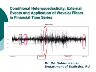
Conditional Heteroscedasticity , External Events and Application of Wavelet Filters in Financial Time Series. Dr. Md . Sabiruzzaman Department of Statistics, RU. Problem Statement.

E N D
Conditional Heteroscedasticity, External Events and Application of Wavelet Filters in Financial Time Series Dr. Md. Sabiruzzaman Department of Statistics, RU
Problem Statement • Financial time series possess some stylized facts like time-varying conditional variance (volatility) and constantunconditional variance, and can be modeled by GARCH family of equations • Analyzing volatility is prior consideration of asset pricing and risk management • External events (policies and crisis) causestemporary (outlier) and permanentchanges (structural break) and the unconditional variance may not constant • Identification of break pointsis important to determine the effect of external events and for proper modeling and forecasting • Tests for structural breaks in volatility (Kokoszka and Leipus, 2000; Andreou and Ghysels, 2002; Sanso et al., 2004; de Pooter and van Dijk, 2004 …) ignore the effect of outliers • An stochastic regime-switching model is not suitable for modeling and forecasting volatility in the presence of structural changes since permanent changes are non-stochastic
Stylized Facts of Financial Time Series • Dependency • Volatility clustering (Manderbolt, 1963) • Time varying conditional variance (Engle,1982) • Constant unconditional variance (Engle,1982) • Persistence (Bollerslev, 1986) • Excess kurtosis (Baillie and Bollerslev,1989) • Asymmetry (Zakoian, 1990) • Long memory (Baillie et al., 1996) • ……
Permanent Change in Variance • By permanent change in variance of financial time series we mean change in the unconditional variance • When a process is observed for a long period of time, permanent changes in the variance may appear as the consequences of external events like natural calamities, economic crisis or policies taken by management (Diebold, 1986; Lamoreaux and Lastraps, 1990; Morana and Beltratti, 2004; Ezaguirre et al., 2004; Rapach and Strauss, 2008 and Karoglou, 2009 ) • Ignorance of structural changes in variance can result as spurious IGARCH or long memory effect (Mikosch and Starica, 2004) • From an economic point of view, structural breaks in financial markets affect fundamental financial indicators (Bates, 2000)
Wavelet Filters • Wavelet transform expresses possibly continuous function in term of discontinuous wavelets. By dilating (stretching) and translating (shifting) a wavelet, we can capture features that are local both in time and frequency • The main feature of wavelet analysis is the possibility to separate out a time series into its constituent multiresolution components. The main algorithm dates back to the work of StephaneMallatin 1988/89 • The discrete wavelet transform (DWT) uses orthogonal transformations to decompose a vector X of length n=2J into vectors of wavelet coefficients D1,D2, . . . ,DJ and A1,A2, . . . ,AJ , where each set of wavelet coefficients contains n/2j data points for j = 1, . . . , J • The approximation coefficients A1,A2, . . . ,AJ contain the low-frequency content, and the detail coefficients D1,D2, . . . ,DJ contain the high-frequency content • By using a small window one looks at high frequency components and by using large window one looks at low-frequency components
Economic Process • Economic and financial systems contain variables that operate on a variety of time scales simultaneously • This implies that the relationship between variables may be different across time scales • Simple example: Securities market contains many traders operating on different time scales • Long view (years), concentrate on market fundamentals • Short view (months), interested in temporary deviations from long-term growth or seasonality • Really short view (hours), interested in ephemeral changes in market behavior • The most important property that wavelets possess for the analysis of economic data is the decomposition by time-scale. Different scale components represent different features of time series. Noise is high frequency components, whereas seasonality is low frequency component.
k=1, 2, …., N where and is an estimator of the long run fourth moment, m4 Here is a proxy volatility measureandinputof the test The asymptotic distribution of is given by where is a Brownian Bridge is a standard Brownian motion Structural Break Detection CUSUM test for dependent process Kokoszka and Leipus (2000) give a consistent CUSUM statistic for detecting variance change in infinite ARCH process
Structural Break Detection CUSUM test for dependent process • The Kokoska and Leipus (KL) test together with ICSS algorithm (Inclan & Tiao, 1994) can be used to detect multiple structural breaks in volatility • The simulation studies of Andreou and Ghysels (2002) and Sanso et al. (2004) extend the use of KL test in more general volatile condition and for detecting multiple breaks but the size distortion problem of KL test is noted
Structural Break Detection Alternative input for KL test based on MODWT • Since a variable is a container of information due to all types of variations: both short-scale and long-scale, square of a variable is, therefore, may be contaminated by some irrelevant components • We suggest a proxy measure of volatility based on maximal overlap discrete wavelet transform (MODWT) coefficients • MODWT is a modified version of DWT given by Percival and Walden (2000) • MODWT is highly redundant but translation invariant transformation • MODWT is energy preserving and properly aligned with features of original series • Unlike DWT, dyadic sample size is not necessarily required for MODWT • Like DWT, analysis of variance (ANOVA) and multiresolution analysis (MRA) is possible with MODWT
Wavelet coefficients at level j associated with scale j Wavelet scaling coefficients represents low frequency components kth wavelet coefficients for different scales Structural Break Detection Alternative input for KL test based on MODWT For given any integer J01, the MODWT wavelet coefficients of {xt} form a (J0+1)N order matrix as
Structural Break Detection Alternative input for KL test based on MODWT The variance of {Xt} can be expressed in terms of multilevel wavelet coefficients as Percival and Walden (2000) show that mean of is and variance As J0 , becomes much smoother and its variance tends to zero and thus for large J0
Structural Break Detection Alternative input for KL test based on MODWT • is the contribution to the energy of {Xt} due to changes at scale j = 2j-1 • The (j,k)th wavelet periodogram, (k = 0, 1, ……, N-1) is the kth contribution to the energy of {Xt} due to changes at scale j • We define an estimator of average variation for different scale at point k based on wavelet periodogram with As J0 increases we will be close to the total variation of the series at point k
Structural Break Detection Alternative input for KL test based on MODWT • Since the choice of J0 depends on length of the sample, we would like to chose js such that as J0 • Fryzlewicz et al. (2003) suggest j=1/2j (j=1, 2, …, J0) • This is a good choice because and the weight j=1/2j is quite well matching with scale j • We call (k=0, 1, …., N-1) the kthmultiscale wavelet periodogram (MSWP) that measures the variation at point k and can be used as input for KL test • The level 1 wavelet periodogram is a special case of MSWP which has been used by many authors to detect outlier and to measure the volatility as well
Structural Break Detection Monte Carlo evidence: Power of the test 2000 simulations from GARCH(1,1) process with a single break (sample size=1024)
Structural Break Detection Monte Carlo evidence: Power of the test 2000 simulations of GARCH(1,1) process with two breaks (sample size=1024)
Structural Break Detection Monte Carlo evidence: Power of the test 2000 simulations of GARCH(1,1) process with two breaks (sample size=1024)
Structural Break Detection Monte Carlo evidence: Size of the test 2000 simulations from GARCH(1,1) process (sample size=1024)
Structural Break Detection Monte Carlo evidence: Spread of detection
Structural Break Detection Monte Carlo evidence: Spread of detection
Structural Break Detection Robustness • KL test is robust to short lived jumps or outliers of moderate size (Andreou and Ghysels, 2002) • Rodrigues and Rubia (2011) show that in presence of bounded outliers KL test is consistent and the asymptotic distribution is invariant • We investigate the extent of robustness of KL test and found that it is heavily sensitive to outliers of large size • It’s a crucial decision which one is to address first- the breaks or the outliers when both are present, because presence of outliers may influence break detection and vice versa • We propose KL test for detecting breaks controlling the effect of outliers by Winsorization. Winsorizationreplaces extreme points with cutoff values
Structural Break Detection Robustness • Standardized sensitivity curve (SV) (Maronna et al., 2006) • Influence function (IF) (Hampel, 1974)
Structural Break Detection Robustness 1000 observations from a GARCH(1,1) process with a single break is simulated and the break detected by KL test is assumed to be the true break point. An outlier is then set before (after) the break, and KL test is applied to the data containing outlier each time. Frequencies of correct detection in 1000 replications for different positions and magnitudes of outliers are reported
Structural Break Detection Robustness 1000 observations from a GARCH(1,1) process with a single break is simulated and the break detected by KL test is assumed to be the true break point. A pair of outliers is then set before (after) the break, and KL test is applied to the data containing outlier each time. Frequencies of correct detection in 1000 replications for different positions and magnitudes of outliers are reported
Structural Break Detection Winsorized KL test Scaled-deviation-Winsorization (Wu and Zuo, 2008): (*) Winsorized KL test: (**)
Structural Break Detection Winsorized KL test • The advantage of scaled-deviation-Winsorization is that by choosing η appropriately it is possible to construct an interval that includes all the good observations. Mathematically, for a small positive quantity ε, we can chose η such that • The chance of mistreating in scaled-deviation-Winsorization technique is low and it can produce the same set of observations as in the original data if no observation is too far from the centre • The fraction of Winsorized points is not fixed but data-dependent
Structural Break Detection Winsorized KL test • Standardized sensitivity curve (SV) • Influence Function (IF)
Structural Break Detection Winsorized KL test The following Theorem confirms that if outliers are bounded through scaled-deviation-Winsorization, the distribution of KL test is invariant
Structural Break Detection Winsorized KL test The following theorem confirms that scaled-deviation-Winsorized KL test is consistent
Structural Break Detection Winsorized KL test 1000 observations from a GARCH(1,1) process with a single break is simulated and the break detected by KL test is assumed to be the true break point. A pair of outliers (6MAD) is then set before (after) the break, and KL test is again applied to Winsorized data each time. Frequencies of correct detection in 10000 replications for different location of outliers are reported
Structural Break Detection Illustration S&P500 daily index and return series over the period January 02, 1980 to September 10, 2010. The vertical lines in the lower panel indicate breaks in long-run variance. Shift 1(17/05/1991): Increase in the index of leading economic indicators, Shift 2(20/07/1997): Asian market crisis, Shift 3(29/04/2003): Iraq invasion and drop in oil prices, Shift 4(23/07/2007): Weakening US housing market
Structural Break Detection Illustration KLSE daily index and return series over the period January 1, 1998 to December 31, 2008. The vertical lines in the lower panel indicate breaks in long-run variance. Shift 1(19/08/1999): Recovery of stock market and real economy, Shift 2(11/10/2001): Tax exemption to encourage investment, Shift 3(17/06/2004): Booming Asian economy, Shift 4(23/02/2007): High global liquidity and increase in fuel price
Modeling Volatility Discrete Breaks • GARCH(1,1) model with k dummies (Lamoureux and Lastrapes, 1990) where zt N(0,1) and • Laumoreux and Lastrapes (1990) only allow the drift to be changed over periods. A straightforward extension can be adding dummies for other parameters as well (see Kim et al., 2010, for example) • To determine the timing of structural breaks, there are model free methods available for detecting break points in volatile series (see Kokoszka and Leipus, 2000, for instance)
Modeling Volatility Stochastic Breaks Switching ARCH (Cai, 1994) The latent variable Stis assumed to follow a first order Markov process with transition probabilities
Modeling Volatility Stochastic Breaks SWARCH model (Hamilton and Susmel, 1994) While Cai (1994) allows the drift of the ARCH process to be varied depending on the latent variable St, Hamilton and Susmel (1994) propose for multiplying by different constant as St indicates changes of regime To avoid the difficulties of estimation due to path dependence Cai (1994) and Hamilton and Susmel (1994) confined themselves to ARCH models
Modeling Volatility Stochastic Breaks Gray (1996) propose that the conditional variance of εt-1, given information at t-2, can be calculated by where is the variance of εt-1, given St-1 = j. Each regime variance is Klaassen (2002) proposes the use of pt-1(St-1 = j), j = 1, …, k, instead of pt-2(St-1 = j), that is, use of information up to time t-1 instead of t-2
Modeling Volatility Stochastic Breaks back back
Modeling Volatility Stochastic Breaks Hass et al. (2004) noted that these models is analytically intractable and, therefore, conditions for covariance stationarity have yet not established. They propose for {St} is a Markov chain with a transition matrix P=[pij]=[P(St=j|St-1=i], i, j = 1, …, k The variance equation is defined as where
Modeling Volatility Discrete vs Stochastic Breaks • Nguyen and Bellahah (2008) find that emerging market experienced multiple breaks in volatility dynamics. The shifts in volatility are associated with events closely related to stock market liberalization, market expansions, and some major economic and political events • Sensier and van Dijk (2004) analyze 214 US macroeconomic time series and find most of the series had an experience of a break within the study period leading to a conclusion that increased stability of economic fluctuations is a widespread phenomenon. They noted that reduced output volatility is primarily accounted for by a reduction in the variance of exogenous shocks hitting the economy. They demonstrate that volatility changes are more appropriately characterized as instantaneous breaks rather than as gradual changes • McConnel and Quiros (2000) documented a structural break in the volatility of US GDP growth. They argue that changes in inventory management techniques have served to stabilize output fluctuations. They also illustrate that widely used regime switching framework is no longer a useful characterization of business cycle movement; the GDP growth is better characterized by a process with structural break in the variance
Identification and verification of break points Fitting a proper break model and test significance of breaks Interested in studying breaks Breaks identified No break identified Not interested in studying breaks Selection of Sample period Verification of Normality, Asymmetry, Memory property and Persistence Segmentation of sample period for in-sample and out-of-sample forecast evaluation Selection of appropriate model based on both in-sample and out-of-sample performance Fitting final model and making inference Steps for Analyzing Volatility in Presence of Breaks
Conclusion • Wavelet filtering facilitate us to decompose a time series variable into its component variations at different time scales and thus, provides an deep insight about the features of the process; use of proposed wavelet-based input improves the size property for the KL test with an assurance that the power is still reasonable • Proposed scaled-deviation-Winsorized KL is robust to detect structural breaks in variance • Stochastic switching volatility models may overlook the structural changes and so, should be utilized with care • Inclusion of observations from the period before a break do not improve forecasting for post break period • Break detection is prior to volatility modeling • Investigate on the properties of MSWP as a volatility measure, like it’s asymptotic distribution, is an interesting subject of future studies
References • Andreou, E. and E. Ghysels (2002). Detecting Multiple Breaks in Financial Market Volatility Dynamics. Journal of Applied Econometrics. 17, 579-600. • Baillie, R.T., T. Bollerslev (1989). The message in daily exchange rates: a conditional variance tale. Journal of Business and Economic Statistics, 7, 297–305 • Baillie, R. T., T. Bollerslev and H. O. Mikkelsen (1996). Fractionally integrated generalized autoregressive conditional heteroskedasticity. Journal of Econometrics. 74: 3-30. • Bollerslev, T. (1986). Generalized autoregressive conditional heteroskedasticity. Journal of Econometrics. 31: 307–327. • Cai, J. (1994). A Markov model of switching-regime ARCH. Journal of Business and Economic Statistics. 12: 309-316. • Charles, A. and O. Darne (2005). Outliers and GARCH models in financial data, Economics Letters, 86, 347-352. • Diebold F. (1988). Empirical Modeling of Exchange Rate Dynamics. Lecture Notes in Economics and Mathematical Systems, New York,N Y: Springer-Verlag • Eizaguirre J. C., J. G. Biscarri and F. P. de Gracia Hidalgo (2004). Structural Changes in Volatility and Stock Market Development: Evidence for Spain. Journal of Banking and Finance. 28: 1745-1773. • Engle, R. F. (1982). Autoregressive conditional heteroskedasticity with estimates of the variance of U.K. inflation. Econometrica. 50: 987–1008. • den Hann W.J. and A. Levin (1997). A Practitioner’s Guide to Robust Covariance Matrix Estimation. Handbook of Statistics. Vol 15. Rao, C.R. and G.S. Maddala (eds). 291-341. • de Pooter, M. and D. van Dijk (2004). Testing for Changes in Volatility in Heteroskedastic Time Series—A Further Examination. Manuscript No. 2004-38/A, Econometrics Institute Research Report. • Doornik, J.A. and M. Ooms (2005). Outlier detection in GARCH models, Technical report, Nuffield College, Oxford.
References • Doornik, J.A. and M. Ooms (2008). Multimodality in GARCH regression models. International Journal of Forecasting, 24, 432-448. • Dueker M. J. (1997). Markov switching in GARCH process and mean-reverting stock-market volatility. Journal of Business and Economic Statistics, 15(1), 26-34. • Franses, P.H. and D. van Dijk (2000). Nonlinear Time Series Model in Empirical Finance, Cambridge University Press, Cambridge. • Franses, P.H. and H. Ghijsels (1999). Aditive outlier, GARCH and forecasting volatility, International Journal of Forecasting, 15, 1-9. • Fryzlewicz, P., S.V. Bellegem and R. von Sachs (2003). Forecasting Non-stationary Time Series by Wavelet Process Modelling. Ann. Inst. Statist. Math. 55(4), 737-764. • Gray, S. F. (1996). Modeling the Conditional Distribution of Interest Rates as a Regime–Switching Process. Journal of Financial Economics. 42: 27–62. • Grossi, L. (2004). Analyzing financial time series through robust estimator. Studies in Nonlinear Dynamics & Economics, 8, article 3. • Haas, M., S. Mittnik and M. S. Paolella (2004). A new approach to Markov-switching GARCH models. Journal of Financial Econometrics. 2(4): 493-530. • Hamilton, J. D. and R. Susmel (1994). Autoregressive conditional heteroskedasticity and changes in regime. Journal of Econometrics. 64: 307-333. • Inclan, C. and G.C. Tiao (1994). Use of Cumulative Sums of Squares for Retrospective Detection of Changes of Variance. Journal of the American Statistical Association, 89, 913-923. • Karoglou M. (2009). Stock Market Efficiency before and after a Financial Liberalisation Reform : Do Breaks in Volatility Dynamics Matter? Journal of Emerging Market Finance. 8: 315-340. • Kim, J., B. Seo and D. Leatham (2010). Structural change in stock price volatility of Asian financial markets. Journal of Economic Research. 15: 1-27. • Klaassen, F. (2002). Improving GARCH Volatility Forecasts with Regime-Switching GARCH. Empirical Economics, 27, 363-394.
References • Kokoszka, P. and R. Leipus (2000). Change-Point Estimation in ARCH Models. Bernoulli 6, 1-28. • Lamoureux, C.G. and W.D. Lastrapes (1990). Persistence in variance, structural change and the GARCH model. Journal of Business and Economic Statistics. 8(2), 225-233. • Mallat, S. (1989). A Theory of Multiresolution Signal Decomposition: The wavelet Representation. IEEE Transactions on Pattern Analysis and Machine Intelligence. 11, 674-693. • Mandelbrot, B. (1963). The variation of certain speculative prices. Journal of Business. 36: 394-419. • McConnell, M and G. Perez-Quiros (2000). Output fluctuation in the United States: what has changed since the early 1980s? American Economic Review. 90: 1464-1476. • Mikosch, T. and C. Stărică (2004). Nonstationarities in Financial Time Series, the Long-Range Dependence, and the IGARCH Effects. Review of Economics and Statistics 86, 378-390. • Newey, W.K. and K.D. West (1994). Automatic Lag Selection in Covariance Matrix Estimation, Review of Economic Studies, 61, 631-653. • Nguyes, D. K. and M. Bellalah (2008). Stock market liberalization, structural breaks and dynamic changes in emerging market volatility. Review of Accounting and Finance. 7(4): 396-411. • Percival, D. B. and A. T. Walden (2000). Wavelet methods for Time Series Analysis. Cambridge University Press, Cambridge, England. • Rapach, D.E. and J.K. Strauss (2008). Structural Breaks and GARCH Models of Exchange rate Volatility. Journal of Applied Econometrics, 23 (1), 65-90. • Rodridgues, P.M.M., Rubia, A. 2011. The effect of additive outliers and measurement errors when testing for structural breaks in variance. Oxford Bulletin of Economics and Statistics. 73(4), 4. • Sansó, A., V. Arragó, and J.L. Carrion (2004). Testing for Change in the Unconditional Variance of Financial Time Series. Revista de EconomiáFinanciera4, 32-53. • Sensier, M. and D. van Dijk (2004). Testing for volatility changes in US macroeconomic time series. Review of Economic and Statistics. 86: 833-839. • Zakoian, J. M. (1990). Threshold heteroskedastic models. CREST, INSEE, Paris, Manuscript.