Download
1 / 12
120 likes | 361 Views
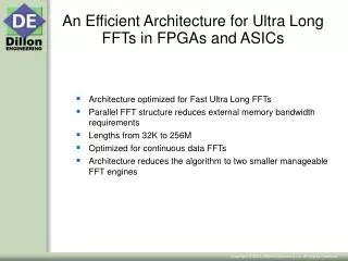
An Efficient Architecture for Ultra Long FFTs in FPGAs and ASICs. Architecture optimized for Fast Ultra Long FFTs Parallel FFT structure reduces external memory bandwidth requirements Lengths from 32K to 256M Optimized for continuous data FFTs

E N D
An Efficient Architecture for Ultra Long FFTs in FPGAs and ASICs • Architecture optimized for Fast Ultra Long FFTs • Parallel FFT structure reduces external memory bandwidth requirements • Lengths from 32K to 256M • Optimized for continuous data FFTs • Architecture reduces the algorithm to two smaller manageable FFT engines
Ultra Long FFTs • An FFT length that exceeds the internal memory requirements of the FPGA or ASIC • System cost can be reduced in moderate length FFTs in designs where the FPGA/ASIC size is driven by the memory requirements. • This architecture puts most of the storage for the FFT off chip in relatively inexpensive SRAM, reducing the system cost. • Ultra Long FFTs have a similar structure to 2D FFTs • Cooley-Tukey algorithm • Minimizes external memory IC count and bandwidth
What Ultra Long FFTs Need The following shows the execution unit (logic) and memory requirement for continuous data FFTs of two lengths: • The logic requirements for a 1M FFT are only double a 1K FFT, while the memory requirements are 1000 times. • Logic for 1M FFT easily fits into large FPGA • Memory requirements exceed what is available even in a large FPGA
Computing N = N1 x N2 The N1 x N2 FFT can be computed as: Computing this for: and Results in: for as desired
N = N1 x N2 Architecture • Three banks of external QDR Memory (single copy each) • Two continuous data FFTs (N1, N2) inside FPGA • Twiddle Multiply provides vector rotation between N2 and N1 FFTs. • Final matrix transpose for normal order output.
QDR SRAM • Simultaneous read/writes (separate address/data bus) allow single bank of memory per memory transpose. • DDR Style I/O so dual clock edge transfer with FPGA results in narrower data path. • Single copy can be kept at each stage while maintaining continuous data flow. • Special address sequence employed so data isn't overwritten in continuous data application. Reduce IC count. • QDR with Virtex II Pro I/O up to 150MHz (read/write) • QDR II with Virtex II Pro I/O up to 200MHz (read/write)
CORDIC For Twiddle Factors Generation • CORDIC produces the sin/cos terms for angle input. • Almost N/2 twiddle factors required. • Very large ROM for FPGA or ASIC. • CORDIC a natural fit, use coordinate product as input.
Matrix Transpose Address Sequence • Allows single copy for each matrix transpose. • Operates on continuous data, one point read/written per clock cycle. • Reduces memory IC count. • Simple logic for sequence generation. • Works for square or rectangular matrices. • Sequence repeats after log2(N) sets. • Write always follows read. • Simple N = N1 x N2 = 8 example: • First and last matrix transpose go left to right in table, second right to left.
Fixed vs. Floating Point • Numbers in radix-2 FFT can grow by log2(N), or 1 bit per butterfly rank. • A 1M FFT can have 20 bits of growth. With 16 bit inputs results would be 36 bits. • Scaling always required in fixed point versions. • Fixed point scaling should be limited to every to every other rank, so 10 times for a 1M FFT producing 26 bit results from 16 bit input. • Floating point FFT maintains precision without overflowing. • Floating Point FFT uses approximately 8 times the logic of a similar precision fixed point version.
80MHz Continuous Data • 1K FFT Engine – 4 butterflies • 512 FFT Engine – 4 butterflies • FFT Engines at 160MHz • QDR memory at 80MHz • Real 14 bit input, complex 24 bit output • Virtex II Pro – Device Usage • Slices - 12,500 • BlockRAM - 144 • MULT18x18 – 88 • Fits in XC2VP40 Virtex II Pro Performance – 512K FFT
Other Uses of Architecture • 2D FFT – Remove first matrix transpose and twiddle multiply. • Variable Length – Use variable length FFTs and dynamic matrix transpose blocks. • Mixed Radix FFTs – Substitute other than radix-2 for 2nd FFT. • Performance increases easy with parallel input radix-2 FFTs and multiple paths to SRAM.
Other Dillon Engineering Resources • ParaCore Architect (parameterized core builder) • DSP Algorithms • Mixed radix FFTs • 2D FFTs for image processing • Fixed or floating-point FFTs • Floating point math library • AES Cryptography • System level DSP • OFDM Transceivers • Radar Processing on single FPGA • Image Compression/Processing • Hardware/Software SOC • High speed Ethernet Appliances • Linux Based SOC in FPGA • MicroBlaze application