Download

1 / 57
610 likes | 790 Views
Rough Sets Tutorial. Contents. Introduction Basic Concepts of Rough Sets Concluding Remarks (Summary, Advanced Topics, References and Further Readings). This is an abridged version of a ppt of 208 slides!!. Introduction.

E N D
Contents • Introduction • Basic Concepts of Rough Sets • Concluding Remarks (Summary, Advanced Topics, References and Further Readings). This is an abridged version of a ppt of 208 slides!!
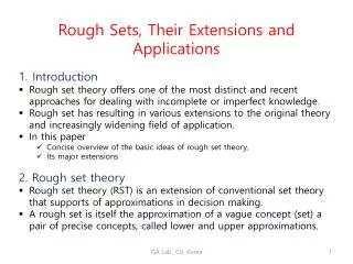
Introduction • Rough set theory was developed by Zdzislaw Pawlak in the early 1980’s. • Representative Publications: • Z. Pawlak, “Rough Sets”, International Journal of Computer and Information Sciences, Vol.11, 341-356 (1982). • Z. Pawlak, Rough Sets - Theoretical Aspect of Reasoning about Data, Kluwer Academic Pubilishers (1991).
Introduction (2) • The main goal of the rough set analysis is induction of approximations of concepts. • Rough sets constitutes a sound basis for KDD. It offers mathematical tools to discover patterns hidden in data. • It can be used for feature selection, feature extraction, data reduction, decision rule generation, and pattern extraction (templates, association rules) etc. • identifies partial or total dependencies in data, eliminates redundant data, gives approach to null values, missing data, dynamic data and others.
Introduction (3) • Fuzzy Sets
Introduction (4) • Rough Sets • In the rough set theory, membership is not the primary concept. • Rough sets represent a different mathematical approach to vagueness and uncertainty.
Introduction (5) • Rough Sets • The rough set methodology is based on the premise that lowering the degree of precision in the data makes the data pattern more visible. • Consider a simple example. Two acids with pKs of respectively pK 4.12 and 4.53 will, in many contexts, be perceived as so equally weak, that they are indiscernible with respect to this attribute. • They are part of a rough set ‘weak acids’ as compared to ‘strong’ or ‘medium’ or whatever other category, relevant to the context of this classification.
Basic Concepts of Rough Sets • Information/Decision Systems (Tables) • Indiscernibility • Set Approximation • Reducts and Core • Rough Membership • Dependency of Attributes
IS is a pair (U, A) U is a non-empty finite set of objects. A is a non-empty finite set of attributes such that for every is called the value set of a. Information Systems/Tables Age LEMS x1 16-30 50 x2 16-30 0 x3 31-45 1-25 x4 31-45 1-25 x5 46-60 26-49 x6 16-30 26-49 x7 46-60 26-49
DS: is the decision attribute(instead of one we can consider more decision attributes). The elements of A are called the condition attributes. Decision Systems/Tables Age LEMS Walk x1 16-30 50 yes x2 16-30 0 no x3 31-45 1-25 no x4 31-45 1-25 yes x5 46-60 26-49 no x6 16-30 26-49 yes x7 46-60 26-49 no
Issues in the Decision Table • The same or indiscernible objects may be represented several times. • Some of the attributes may be superfluous.
Indiscernibility • The equivalence relation A binary relation which is reflexive (xRx for any object x) , symmetric (if xRy then yRx), and transitive (if xRy and yRz then xRz). • The equivalence class of an element consists of all objects such that xRy.
Indiscernibility (2) • Let IS = (U, A) be an information system, then with any there is an associated equivalence relation: where is called the B-indiscernibility relation. • If then objects x and x’ are indiscernible from each other by attributes from B. • The equivalence classes of the B-indiscernibility relation are denoted by
The non-empty subsets of the condition attributes are {Age}, {LEMS}, and {Age, LEMS}. IND({Age}) = {{x1,x2,x6}, {x3,x4}, {x5,x7}} IND({LEMS}) = {{x1}, {x2}, {x3,x4}, {x5,x6,x7}} IND({Age,LEMS}) = {{x1}, {x2}, {x3,x4}, {x5,x7}, {x6}}. An Example of Indiscernibility Age LEMS Walk x1 16-30 50 yes x2 16-300 no x3 31-45 1-25 no x4 31-451-25 yes x5 46-60 26-49 no x6 16-30 26-49 yes x7 46-60 26-49 no
Observations • An equivalence relation induces a partitioning of the universe. • The partitions can be used to build new subsets of the universe. • Subsets that are most often of interest have the same value of the decision attribute. It may happen, however, that a concept such as “Walk” cannot be defined in a crisp manner.
Set Approximation • Let T = (U, A) and let and We can approximate X using only the information contained in B by constructing the B-lower and B-upper approximations of X, denoted and respectively, where
Set Approximation (2) • B-boundary region of X, consists of those objects that we cannot decisively classify into X in B. • B-outside region of X, consists of those objects that can be with certainty classified as not belonging to X. • A set is said to be roughif its boundary region is non-empty, otherwise the set is crisp.
Let W = {x | Walk(x) = yes}. The decision class, Walk, is rough since the boundary region is not empty. An Example of Set Approximation Age LEMS Walk x1 16-30 50 yes x2 16-30 0 no x3 31-45 1-25 no x4 31-45 1-25 yes x5 46-60 26-49 no x6 16-30 26-49 yes x7 46-60 26-49 no
An Example of Set Approximation (2) {{x2}, {x5,x7}} {{x3,x4}} yes AW {{x1},{x6}} yes/no no
Lower & Upper Approximations U U/R R : subset of attributes Set X
Lower & Upper Approximations (2) Upper Approximation: Lower Approximation:
Lower & Upper Approximations (3) The indiscernibility classes defined by R = {Headache, Temp.} are {u1}, {u2}, {u3}, {u4}, {u5, u7}, {u6, u8}. X1 = {u | Flu(u) = yes} = {u2, u3, u6, u7} RX1 = {u2, u3} = {u2, u3, u6, u7, u8, u5} X2 = {u | Flu(u) = no} = {u1, u4, u5, u8} RX2 = {u1, u4} = {u1, u4, u5, u8, u7, u6}
Lower & Upper Approximations (4) R = {Headache, Temp.} U/R = { {u1}, {u2}, {u3}, {u4}, {u5, u7}, {u6, u8}} X1 = {u | Flu(u) = yes} = {u2,u3,u6,u7} X2 = {u | Flu(u) = no} = {u1,u4,u5,u8} X2 X1 RX1 = {u2, u3} = {u2, u3, u6, u7, u8, u5} u2 u7 u5 u1 RX2 = {u1, u4} = {u1, u4, u5, u8, u7, u6} u6 u8 u3 u4
Properties of Approximations implies and
Properties of Approximations (2) where -X denotes U - X.
Four Basic Classes of Rough Sets • X is roughly B-definable, iff and • X is internally B-undefinable, iff and • X is externally B-undefinable, iff and • X is totally B-undefinable, iff and
Accuracy of Approximation where |X| denotes the cardinality of Obviously If X is crisp with respect to B. If X is rough with respect to B.
Issues in the Decision Table • The same or indiscernible objects may be represented several times. • Some of the attributes may be superfluous (redundant). That is, their removal cannot worsen the classification.
Reducts • Keep only those attributes that preserve the indiscernibility relation and, consequently, set approximation. • There are usually several such subsets of attributes and those which are minimal are called reducts.
Dispensable & Indispensable Attributes Let Attribute c is dispensable in T if , otherwise attribute c is indispensable in T. The C-positive region of D:
Independent • T = (U, C, D) is independent if all are indispensable in T.
Reduct & Core • The set of attributes is called a reduct of C, if T’ = (U, R, D) is independent and • The set of all the condition attributes indispensable in T is denoted by CORE(C). where RED(C) is the set of all reducts of C.
An Example of Reducts & Core Reduct1 = {Muscle-pain,Temp.} Reduct2 = {Headache, Temp.} CORE = {Headache,Temp} {MusclePain, Temp} = {Temp}
Discernibility Matrix (relative to positive region) • Let T = (U, C, D) be a decision table, with By a discernibility matrix of T, denoted M(T), we will mean matrix defined as: for i, j = 1,2,…,n such that or belongs to the C-positive region of D. • is the set of all the condition attributes that classify objects ui and uj into different classes.
Discernibility Matrix (relative to positive region) (2) • The equation is similar but conjunction is taken over all non-empty entries of M(T) corresponding to the indices i, j such that or belongs to the C-positive region of D. • denotes that this case does not need to be considered. Hence it is interpreted as logic truth. • All disjuncts of minimal disjunctive form of this function define the reducts of T (relative to the positive region).
Discernibility Function (relative to objects) • For any where (1) is the disjunction of all variables a such that if (2) if (3) if Each logical product in the minimal disjunctive normal form (DNF) defines a reduct of instance
Examples of Discernibility Matrix In order to discern equivalence classes of the decision attribute d, to preserve conditions described by the discernibility matrix for this table No a b c d u1 a0 b1 c1 y u2 a1 b1 c0 n u3 a0 b2 c1 n u4 a1 b1 c1 y u1 u2 u3 C = {a, b, c} D = {d} u2 u3 u4 a,c b c a,b Reduct = {b, c}
Examples of Discernibility Matrix (2) u1 u2 u3 u4 u5 u6 u2 u3 u4 u5 u6 u7 b,c,d b,c b b,d c,d a,b,c,d a,b,c a,b,c,d a,b,c,d a,b,c a,b,c,d a,b,c,d a,b c,d c,d Core = {b} Reduct1 = {b,c} Reduct2 = {b,d}
What Are Issues of Real World ? • Very large data sets • Mixed types of data (continuous valued, symbolic data) • Uncertainty (noisy data) • Incompleteness (missing, incomplete data) • Data change • Use of background knowledge
A Rough Set Based KDD Process • Discretization based on RS and Boolean Reasoning (RSBR). • Attribute selection based RS with Heuristics (RSH). • Rule discovery by Generalization Distribution Table (GDT)-RS. KDD: Knowledge Discovery and Datamining
Summary • Rough sets offers mathematical tools and constitutes a sound basis for KDD. • We introduced the basic concepts of (classical) rough set theory.
Advanced Topics(to deal with real world problems) • Recent extensions of rough set theory (rough mereology: approximate synthesis of objects) have developed new methods for decomposition of large datasets, data mining in distributed and multi-agent systems, and fusion of information granules to induce complex information granule approximation.
Advanced Topics (2)(to deal with real world problems) • Combining rough set theory with logic (including non-classical logic), ANN, GA, probabilistic and statistical reasoning, fuzzy set theory to construct a hybrid approach.
References and Further Readings • Z. Pawlak, “Rough Sets”, International Journal of Computer and Information Sciences, Vol.11, 341-356 (1982). • Z. Pawlak, Rough Sets - Theoretical Aspect of Reasoning about Data, Kluwer Academic Publishers (1991). • L. Polkowski and A. Skowron (eds.) Rough Sets in Knowledge Discovery, Vol.1 and Vol.2., Studies in Fuzziness and Soft Computing series, Physica-Verlag (1998). • L. Polkowski and A. Skowron (eds.) Rough Sets and Current Trends in Computing, LNAI 1424. Springer (1998). • T.Y. Lin and N. Cercone (eds.), Rough Sets and Data Mining, Kluwer Academic Publishers (1997). • K. Cios, W. Pedrycz, and R. Swiniarski, Data Mining Methods for Knowledge Discovery, Kluwer Academic Publishers (1998).
References and Further Readings • R. Slowinski, Intelligent Decision Support, Handbook of Applications and Advances of the Rough Sets Theory, Kluwer Academic Publishers (1992). • S.K. Pal and S. Skowron (eds.) Rough Fuzzy Hybridization: A New Trend in Decision-Making, Springer (1999). • E. Orlowska (ed.) Incomplete Information: Rough Set Analysis, Physica-Verlag (1997). • S. Tsumolto, et al. (eds.) Proceedings of the 4th International Workshop on Rough Sets, Fuzzy Sets, and Machine Discovery, The University of Tokyo (1996). • J. Komorowski and S. Tsumoto (eds.) Rough Set Data Analysis in Bio-medicine and Public Health, Physica-Verlag (to appear).
References and Further Readings • W. Ziarko, “Discovery through Rough Set Theory”, Knowledge Discovery: viewing wisdom from all perspectives, Communications of the ACM, Vol.42, No. 11 (1999). • W. Ziarko (ed.) Rough Sets, Fuzzy Sets, and Knowledge Discovery, Springer (1993). • J. Grzymala-Busse, Z. Pawlak, R. Slowinski, and W. Ziarko, “Rough Sets”, Communications of the ACM, Vol.38, No. 11 (1999). • Y.Y. Yao, “A Comparative Study of Fuzzy Sets and Rough Sets”, Vol.109, 21-47, Information Sciences (1998). • Y.Y. Yao, “Granular Computing: Basic Issues and Possible Solutions”, Proceedings of JCIS 2000, Invited Session on Granular Computing and Data Mining, Vol.1, 186-189 (2000).
References and Further Readings • N. Zhong, A. Skowron, and S. Ohsuga (eds.), New Directions in Rough Sets, Data Mining, and Granular-Soft Computing, LNAI 1711, Springer (1999). • A. Skowron and C. Rauszer, “The Discernibility Matrices and Functions in Information Systems”, in R. Slowinski (ed) Intelligent Decision Support, Handbook of Applications and Advances of the Rough Sets Theory, 331-362, Kluwer (1992). • A. Skowron and L. Polkowski, “Rough Mereological Foundations for Design, Analysis, Synthesis, and Control in Distributive Systems”, Information Sciences, Vol.104, No.1-2, 129-156, North-Holland (1998). • C. Liu and N. Zhong, “Rough Problem Settings for Inductive Logic Programming”, in N. Zhong, A. Skowron, and S. Ohsuga (eds.), New Directions in Rough Sets, Data Mining, and Granular-Soft Computing, LNAI 1711, 168-177, Springer (1999).
References and Further Readings • J.Z. Dong, N. Zhong, and S. Ohsuga, “Rule Discovery by Probabilistic Rough Induction”, Journal of Japanese Society for Artificial Intelligence, Vol.15, No.2, 276-286 (2000). • N. Zhong, J.Z. Dong, and S. Ohsuga, “GDT-RS: A Probabilistic Rough Induction System”, Bulletin of International Rough Set Society, Vol.3, No.4, 133-146 (1999). • N. Zhong, J.Z. Dong, and S. Ohsuga,“Using Rough Sets with Heuristics for Feature Selection”, Journal of Intelligent Information Systems (to appear). • N. Zhong, J.Z. Dong, and S. Ohsuga, “Soft Techniques for Rule Discovery in Data”, NEUROCOMPUTING, An International Journal, Special Issue on Rough-Neuro Computing (to appear).
References and Further Readings • H.S. Nguyen and S.H. Nguyen, “Discretization Methods in Data Mining”, in L. Polkowski and A. Skowron (eds.) Rough Sets in Knowledge Discovery, Vol.1, 451-482, Physica-Verlag (1998). • T.Y. Lin, (ed.) Journal of Intelligent Automation and Soft Computing, Vol.2, No. 2, Special Issue on Rough Sets (1996). • T.Y. Lin (ed.) International Journal of Approximate Reasoning, Vol.15, No. 4, Special Issue on Rough Sets (1996). • Z. Ziarko (ed.) Computational Intelligence, An International Journal, Vol.11, No. 2, Special Issue on Rough Sets (1995). • Z. Ziarko (ed.) Fundamenta Informaticae, An International Journal, Vol.27, No. 2-3, Special Issue on Rough Sets (1996).
References and Further Readings • A. Skowron et al. (eds.) NEUROCOMPUTING, An International Journal, Special Issue on Rough-Neuro Computing (to appear). • A. Skowron, N. Zhong, and N. Cercone (eds.) Computational Intelligence, An International Journal, Special Issue on Rough Sets, Data Mining, and Granular Computing (to appear). • J. Grzymala-Busse, R. Swiniarski, N. Zhong, and Z. Ziarko (eds.) International Journal of Applied Mathematics and Computer Science, Special Issue on Rough Sets and Its Applications (to appear).