Download
1 / 61
660 likes | 1.04k Views
Stoner-Wohlfarth Theory. “A Mechanism of Magnetic Hysteresis in Heterogenous Alloys” Stoner E C and Wohlfarth E P (1948), Phil. Trans. Roy. Soc. A240 :599–642 Prof. Bill Evenson , Utah Valley University. E.C. Stoner, c. 1934 . E. C. Stoner, F.R.S. and E. P. Wohlfarth (no photo)

E N D
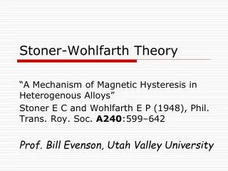
Stoner-Wohlfarth Theory “A Mechanism of Magnetic Hysteresis in Heterogenous Alloys” Stoner E C and Wohlfarth E P (1948), Phil. Trans. Roy. Soc. A240:599–642 Prof. Bill Evenson, Utah Valley University
E.C. Stoner, c. 1934 E. C. Stoner, F.R.S. and E. P. Wohlfarth (no photo) (Note: F.R.S. = “Fellow of the Royal Society”) Courtesy of AIP Emilio Segre Visual Archives TU-Chemnitz
Stoner-Wohlfarth Motivation • How to account for very high coercivities • Domain wall motion cannot explain • How to deal with small magnetic particles (e.g. grains or imbedded magnetic clusters in an alloy or mixture) • Sufficiently small particles can only have a single domain TU-Chemnitz
Hysteresis loop Mr = Remanence Ms = Saturation Magnetization Hc = Coercivity TU-Chemnitz
Domain Walls • Weiss proposed the existence of magnetic domains in 1906-1907 • What elementary evidence suggests these structures? www.cms.tuwien.ac.at/Nanoscience/Magnetism/magnetic-domains/magnetic_domains.htm TU-Chemnitz
Stoner-Wohlfarth Problem • Single domain particles (too small for domain walls) • Magnetization of a particle is uniform and of constant magnitude • Magnetization of a particle responds to external magnetic field and anisotropy energy TU-Chemnitz
Not Stoner Theory of BandFerromagnetism The Stoner-Wohlfarth theory of hysteresis does not refer to the Stoner (or Stoner-Slater) theory of band ferromagnetism or to such terms as “Stoner criterion”, “Stoner excitations”, etc. TU-Chemnitz
Small magnetic particles TU-Chemnitz
Why are we interested? (since 1948!) Magnetic nanostructures! Can be single domain, uniform/constant magnetization, no long-range order between particles, anisotropic. TU-Chemnitz
Physics in SW Theory • Classical e & m (demagnetization fields, dipole) • Weiss molecular field (exchange) • Ellipsoidal particles for shape anisotropy • Phenomenological magnetocrystalline and strain anisotropies • Energy minimization TU-Chemnitz
Outline of SW 1948 (1) • 1. Introduction • review of existing theories of domain wall motion (energy, process, effect of internal stress variations, effect of changing domain wall area – especially due to nonmagnetic inclusions) • critique of boundary movement theory • Alternative process: rotation of single domains (small magnetic particles – superparamagnetism) – roles of magneto-crystalline, strain, and shape anisotropies TU-Chemnitz
Outline of SW 1948 (2) • 2. Field Dependence of Magnetization Direction of a Uniformly Magnetized Ellipsoid – shape anisotropy • 3. Computational Details • 4. Prolate Spheroid Case • 5. Oblate Spheroid and General Ellipsoid TU-Chemnitz
Outline of SW 1948 (3) • 6. Conditions for Single Domain Ellipsoidal Particles • 7. Physical Implications • types of magnetic anisotropy • magnetocrystalline, strain, shape • ferromagnetic materials • metals & alloys containing FM impurities • powder magnets • high coercivity alloys TU-Chemnitz
Units, Terminology, Notation E.g. • Gaussian e-m units • 1 Oe = 1000/4π × A/m • Older terminology • “interchange interaction energy” = “exchange interaction energy” • Older notation • I0 = magnetization vector TU-Chemnitz
Mathematical Starting Point • Applied field energy • Anisotropy energy • Total energy (what should we use?) (later, drop constants) TU-Chemnitz
MAGNETIC ANISOTROPY • Shape anisotropy (dipole interaction) • Strain anisotropy • Magnetocrystalline anisotropy • Surface anisotropy • Interface anisotropy • Chemical ordering anisotropy • Spin-orbit interaction • Local structural anisotropy TU-Chemnitz
Ellipsoidal particles This gives shape anisotropy – from demagnetizing fields (to be discussed later if there is time). Spherical particles would not have shape anisotropy, but would have magnetocrystalline and strain anisotropy – leading to the same physics with redefined parameters. TU-Chemnitz
Ellipsoidal particles We will look at one ellipsoidal particle, then average over a random orientation of particles. The transverse components of mag-netization will cancel, and the net magnetiza-tion can be calculated as the component along the applied field direction. TU-Chemnitz
Demagnetizing fields → anisotropy from Bertotti TU-Chemnitz
Prolate and Oblate Spheroids These show all the essential physics of the more general ellipsoid. TU-Chemnitz
How do we get hysteresis? I0 Easy Axis H TU-Chemnitz
SW Fig. 1 – important notation One can prove (SW outline the proof in Sec. 5(ii)) that for ellipsoids of revolution H, I0, and the easy axis all lie in a plane. TU-Chemnitz
No hysteresis for oblate case I0 Easy Axis 360o degenerate H TU-Chemnitz
Mathematical Starting Point - again • Applied field energy • Anisotropy energy • Total energy (later, drop constants) TU-Chemnitz
Dimensionless variables Total energy: normalize to and drop constant term. Dimensionless energy is then TU-Chemnitz
Energy surface for fixed θ θ = 10o TU-Chemnitz
Stationary points (max & min) θ = 10o TU-Chemnitz
SW Fig. 2 TU-Chemnitz
SW Fig. 3 TU-Chemnitz
Examples in Maple (This would be easy to do with Mathematica, also.) [SW_Lectures_energy_surfaces.mw] TU-Chemnitz
Calculating the Hysteresis Loop TU-Chemnitz
from Blundell TU-Chemnitz
SW Fig. 6 TU-Chemnitz
Examples in Maple [SW_Lectures_hysteresis.mw] TU-Chemnitz
Hsw and Hc TU-Chemnitz
Hysteresis Loops: 0-45o and 45-90o – symmetries from Blundell TU-Chemnitz
Hysteresis loop for θ = 90o from Jiles TU-Chemnitz
Hysteresis loop for θ = 0o from Jiles TU-Chemnitz
Hysteresis loop for θ = 45o from Jiles TU-Chemnitz
Average over Orientations TU-Chemnitz
SW Fig. 7 TU-Chemnitz
Part 2 • Conditions for large coercivity • Applied field • Various forms of magnetic anisotropy • Conditions for single-domain ellipsoidal particles TU-Chemnitz
DemagnetizationCoefficients: large Hc possible SW Fig. 8 m=a/b I0~103 TU-Chemnitz
Applied Field, H • Important! This is the total field experienced by an individual particle. It must include the field due to the magnetizations of all the other particles around the one we calculate! TU-Chemnitz
Magnetic Anisotropy • Regardless of the origin of the anisotropy energy, the basic physics is approximately the same as we have calculated for prolate spheroids. • This is explicitly true for • Shape anisotropy • Magnetocrystalline anisotropy (uniaxial) • Strain anisotropy TU-Chemnitz
Demagnetizing Field Energy • Energetics of magnetic media are very subtle. is the “demagnetizing field” from Blundell TU-Chemnitz
Demagnetizing fields → anisotropy from Bertotti TU-Chemnitz
How does depend on shape? is extremely complicated for arbitrarily shaped ferromagnets, but relatively simple for ellipsoidal ones. And in principal axis coordinate system for the ellipsoid, TU-Chemnitz
Ellipsoids (Gaussian units) (SI units) TU-Chemnitz
Examples • Sphere • Long cylindrical rod • Flat plate TU-Chemnitz