Download
1 / 29
300 likes | 636 Views
I X. Hilbert Huang Transform (HHT). 為中研院黃鍔院士於 1998 年提出. 黃鍔院士的生平可參考. http://sec.ncu.edu.tw/E-News/ detail.php?SelectPaperPK=14&SelectReportPK=115&Pic=15. References.

E N D
IX. Hilbert Huang Transform (HHT) 為中研院黃鍔院士於 1998 年提出 黃鍔院士的生平可參考 http://sec.ncu.edu.tw/E-News/ detail.php?SelectPaperPK=14&SelectReportPK=115&Pic=15 References [1] N. E. Huang, Z. Shen, S. R. Long, M. C. Wu, H. H. Shih, Q. Zheng, N. C. Yen, C. C. Tung, and H. H. Liu, “The empirical mode decomposition and the Hilbert spectrum for nonlinear and non-stationary time series analysis,” Proc. R. Soc. Lond. A, vol. 454, pp. 903-995, 1998. [2] N. E. Huang and S. Shen, Hilbert-Huang Transform and Its Applications, World Scientific, Singapore, 2005. (PS: 謝謝 2007 年修課的趙逸群同學和王文阜同學)
9-A 觀念起源 另一種分析 instantaneous frequency 的方式: Hilbert transform Hilbert transform or H(f) j f-axis f = 0 -j
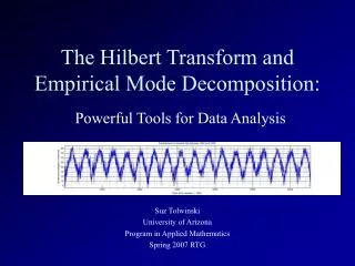
Applications of the Hilbert Transform analytic signal another way to define the instantaneous frequency: where Example:
Problem of using Hilbert transforms to determine the instantaneous frequency: This method is only good for cosine and sine functions with single component. Not suitable for (1) complex function (2) non-sinusoid-like function (3) multiple components Example:
Hilbert-Huang transform 的基本精神: 先將一個信號分成多個 sinusoid-like components + trend (和 Fourier analysis 不同的地方在於,這些 sinusoid-like components 的 period 和 amplitude 可以不是固定的) 再運用 Hilbert transform (或 STFT,number of zero crossings) 來分析每個 components 的 instantaneous frequency 完全不需用到 Fourier transform
9-B Intrinsic Mode Function (IMF) 條件 (1) The number of extremes and the number of zero-crossings must either equal or differ at most by one. (2) At any point, the mean value of the envelope defined by the local maxima and the envelope defined by the local minima is near to zero.
2 1 0 -1 9-C Hilbert Huang Transform 的流程 Steps 1~8 被稱為 Empirical Mode Decomposition (EMD) (Step 1) Initial: y(t) = x(t), (x(t) is the input) n = 1, k = 1 (Step 2) Find the local peaks y(t)
IMF 1; iteration 0 2 1 0 -1 (Step 3) Connect local peaks 通常使用 B-spline,尤其是 cubic B-spline來連接 (參考附錄十)
IMF 1; iteration 0 2 1 0 -1 (Step 4) Find the local dips (Step 5) Connect the local dips
IMF 1; iteration 0 2 1 0 -1 (Step 6-1) Compute the mean (pink line)
1.5 1 0.5 0 -0.5 -1 -1.5 (Step 6-2) Compute the residue
(Step 7) Check whether hk(t) is an intrinsic modefunction (IMF) (1) 檢查是否 local maximums 皆大於 0 local minimums 皆小於 0 (2) 上封包: u1(t), 下封包: u0(t) 檢查是否 for all t If they are satisfied (or k ≧ K), set cn(t) = hk(t) and continue to Step 8 cn(t) is the nth IMF of x(t). If not, set y(t) = hk(t), k = k + 1, and repeat Steps 2~6 (為了避免無止盡的迴圈,可以定 k 的上限 K)
(Step 8) Calculate and check whether x0(t) is a function with no more thanone extreme point. If not, set n = n+1, y(t) = x0(t) and repeat Steps 2~7 If so, the empirical mode decomposition is completed. Step 8 Step 7 Y x0(t) has only 0 or 1 extreme? hk(t) is an IMF? Y Step 9 Step 1 Steps 2~6 N trend N
(Step 9) Find the instantaneous frequency for each IMF cs(t) (s = 1, 2, …, n). Method 1: Using the Hilbert transform Method 2:Calculating the STFT for cs(t). Method 3: Furthermore, we can also calculate the instantaneous frequency fromthe number of zero-crossings directly. instantaneous frequency Fs(t) of cs(t)
邊界處理的問題: 目前尚未有一致的方法,可行的方式有 (1) 只使用非邊界的 extreme points (2) 將最左、最右的點當成是 extreme points (3) 預測邊界之外的 extreme points 的位置和大小
9-D Example Example 1 After Step 6
IMF1 IMF2 x0(t)
Example 2 hum signal IMF1 IMF2
IMF3 IMF4 IMF5 IMF6
IMF7 IMF8 IMF9 IMF10
IMF11 x0(t)
9-E Advantages and Disadvantages Advantages (1) 避免了複雜的數學理論分析 (2) 可以找到一個 function 的「趨勢」 (3) 和其他的時頻分析一樣,可以分析頻率會隨著時間而改變的信號 (4) 適合於 Climate analysis Economical data Geology Acoustics Music signal
Disadvantages (1) 除了 x0(t) 可以看出一個信號的「趨勢」之外, 其他的 intrinsic mode functions (IMFs) 缺乏嚴謹的物理意義 甚至可能偶而會出現後面的 IMF 的instantaneous frequency 反而高於前面的 IMF 的情形 (2) 運算時間有時反而會比 STFT 來得多 (因為需要兩個迴圈) (3) 即使是 IMF,instantaneous frequency 未必能由 Hilbert transform 完美 的分析出來 用 zero-crossing 算出的 instantaneous frequency必為 1/2 的倍數,且不夠精確
結論 當信號含有「趨勢」 或是由少數幾個 sinusoid functions 所組合而成,而且這些sinusoid functions 的 amplitudes 相差懸殊時,可以用 HHT 來分析 然而,對於其他的情形,用其他的 time-frequency analysis 或是用 wavelet 較為適合
附錄十 Interpolation and the B-Spline Suppose that the sampling points are t1, t2, t3, …, tNand we have known the values of x(t) at these sampling points. There are several ways for interpolation. (1) The simplest way: Using the straight lines (i.e., linear interpolation) t1 t2 t3 t4
(2) Lagrange interpolation 指的是連乘符號, (3) Polynomial interpolation solve a1, a2, a3, ……, aN from
(4) Lowpass FilterInterpolation 適用於 sampling interval 為固定的情形 tn+1 tn = tfor all n discrete time Fourier transform lowpass mask X1(f) X(f) x(tn) inverse discrete time Fourier transform x(t)
(5) B-Spline Interpolation B-spline 簡稱為 spline for tn < t < tn+1 otherwise m = 1: linear B-spline m = 2: quadratic B-spline m = 3: cubic B-spline (通常使用)
在 Matlab 當中,可以用 “spline” 這個指令來做 interpolation (註: Matlab 用的是 cubic B-spline) Example: Generates a sine-like spline curve and samples it over a finer mesh: x = 0:10; y = sin(x); xx = 0:0.1:10; yy = spline(x,y,xx); plot(x,y,'o',xx,yy)