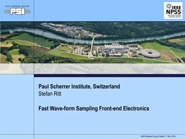
Paul Scherrer Institute, Switzerland
Stefan Ritt. Paul Scherrer Institute, Switzerland. Fast Wave-form Sampling Front-end Electronics. Prologue. RTSD Luncheon. Undersampling of signals. Undersampling: Acquisition of signals with sampling rates ≪ 2 * highest frequency in signal. Image Processing. Waveform Processing. Agenda.

Paul Scherrer Institute, Switzerland
E N D
Presentation Transcript
Stefan Ritt Paul Scherrer Institute, Switzerland Fast Wave-form Sampling Front-end Electronics NSS Refresher Course, Seattle,
Prologue RTSD Luncheon NSS Refresher Course, Seattle,
Undersampling of signals Undersampling: Acquisition of signals with sampling rates ≪ 2 * highest frequency in signal Image Processing Waveform Processing NSS Refresher Course, Seattle,
Agenda What is the problem? Tool to solve it 1 2 3 What else can we do with that tool? NSS Refresher Course, Seattle,
What is the problem? 1 NSS Refresher Course, Seattle,
Signals in particle physics Scintillators (Plastic, Crystals, Noble Liquids, …) Photomultiplier (PMT) Scintillator Particle HV 10 – 100 ns Wire chambersStraw tubes HV Silicon Germanium 1 – 10 ms NSS Refresher Course, Seattle,
Measure precise timing: ToF-PET Positron Emission Tomography Time-of-Flight PET d Dt e.g. d=1 cm → Dt = 67 ps d ~ c/2 * Dt NSS Refresher Course, Seattle,
Traditional DAQ in Particle Physics Threshold ADC ~MHz + - TDC (Clock) Threshold NSS Refresher Course, Seattle,
Signal discrimination Single Threshold Multiple Thresholds Constant Fraction (CFD) Inverter & Attenuator T1 Threshold S T2 0 Adder T3 Delay “Time-Walk” T1 T2 T3 NSS Refresher Course, Seattle,
Influence of noise Voltage noise causes timing jitter ! Signal Low pass filter Noise Fourier Spectrum Low pass filter (shaper) reduces noise while maintaining most of the signal NSS Refresher Course, Seattle,
Noise limited time accuracy All values in this talk are s (RMS) ! FHWM = 2.35 x s Most today’s TDCs have ~20 ps LSB How can we do better ? NSS Refresher Course, Seattle,
Noise limited time accuracy NSS Refresher Course, Seattle,
Switching to Waveform digitizing • Advantages: • General trend in signal processing (“Software Defined Radio”) • Less hardware (Only ADC and FPGA) • Algorithms can be complex (peak finding, peak counting, waveform fitting) • Algorithms can be changed without changing the hardware • Storage of full waveforms allow elaborate offline analysis SDR ADC ~100 MHz FPGA NSS Refresher Course, Seattle,
Example: CFG in FPGA FPGA S 0 Adder Delay * (-0.3) Adder Look-up Table (LUT) 8-bit address 8-bit data + >0 Latch AND ≤ 0 Clock Delay NSS Refresher Course, Seattle,
Nyquist-Shannon Sampling Theorem fsignal < fsampling /2 fsignal > fsampling /2 NSS Refresher Course, Seattle,
Limits of waveform digitizing • Aliasing Occurs if fsignal > 0.5 * fsampling • Features of the signal can be lost (“pile-up”) • Measurement of time becomes hard • ADC resolution limits energy measurement • Need very fast high resolutionADC NSS Refresher Course, Seattle,
What are the fastest detectors? • Micro-Channel-Plates (MCP) • Photomultipliers with thousands of tiny channels (3-10 mm) • Typical gain of 10,000 per plate • Very fast rise time down to 70 ps • 70 ps rise time 4-5 GHz BW 10 GSPS • SiPMs (Silicon PMTs) are also getting < 100 ps J. Milnes, J. Howoth, Photek NSS Refresher Course, Seattle,
Can it be done with FADCs? 8 bits – 3 GS/s – 1.9 W 24 Gbits/s 10 bits – 3 GS/s – 3.6 W 30 Gbits/s 12 bits – 3.6 GS/s – 3.9 W 43.2 Gbits/s 14 bits – 0.4 GS/s – 2.5 W 5.6 Gbits/s PX1500-4: 2 Channel3 GS/s8 bits 24x1.8 Gbits/s 1.8 GHz! 1-10 k$ / channel What about 1000+ Channels? • Requires high-end FPGA • Complex board design • High FPGA power ADC12D1X00RB: 1 Channel 1.8 GS/s 12 bits V1761: 2 Channels, 4 GS/s, 10 bits NSS Refresher Course, Seattle,
Tool to solve it 2 NSS Refresher Course, Seattle,
Switched Capacitor Array (Analog Memory) 10-100 mW 0.2-2 ns Inverter “Domino” ring chain IN Waveform stored Out FADC 33 MHz Clock Shift Register “Time stretcher” GHz MHz NSS Refresher Course, Seattle,
IN Out Clock Time Stretch Ratio (TSR) dts • Typical values: • dts = 0.5 ns (2 GSPS) • dtd = 30 ns (33 MHz)→ TSR = 60 dtd NSS Refresher Course, Seattle,
Triggered Operation sampling digitization sampling digitization Sampling Windows * TSR lost events Dead time = Sampling Window ∙ TSR (e.g. 100 ns ∙ 60 = 6 ms) Chips usually cannot sample during readout ⇒ “Dead Time” Technique only works for “events” and “triggers” NSS Refresher Course, Seattle,
Time resolution limit of SCA PCB Chip Det. Cpar NSS Refresher Course, Seattle,
Bandwidth STURM2 (32 sampling cells) G. Varner, Dec. 2009 NSS Refresher Course, Seattle,
How is timing resolution affected? today: optimized SNR: next generation: - high frequency noise - quantization noise NSS Refresher Course, Seattle,
Timing Nonlinearity Bin-to-bin variation:“differential timing nonlinearity” Difference along the whole chip:“integral timing nonlinearity” Nonlinearity comes from size (doping)of inverters and is stable over time→ can be calibrated Residual random jitter:1-2 ps RMS beats best TDC Recently achieved with new calibration method http://arxiv.org/abs/1405.4975 Dt Dt Dt Dt Dt NSS Refresher Course, Seattle,
First Switched Capacitor Arrays IEEE Transactions on Nuclear Science, Vol. 35, No. 1, Feb. 1988 50 MSPS in 3.5 mm CMOS process NSS Refresher Course, Seattle,
Switched Capacitor Arrays for Particle Physics E. Delagnes D. Breton CEA Saclay H. Frisch et al., Univ. Chicago G. Varner, Univ. of Hawaii LABRADOR3 STRAW3 TARGET AFTER SAM NECTAR0 PSEC1 - PSEC4 • 0.13 mm IBM • Large Area Picosecond Photo-Detectors Project (LAPPD) • 0.35 mm AMS • T2K TPC, Antares, Hess2, CTA • 0.25 mm TSMC • Many chips for different projects(Belle, Anita, IceCube …) matacq.free.fr psec.uchicago.edu www.phys.hawaii.edu/~idlab/ DRS3 DRS4 DRS1 DRS2 • 0.25 mm UMC • Universal chip for many applications • MEG experiment, MAGIC, Veritas, TOF-PET SR R. Dinapoli PSI, Switzerland drs.web.psi.ch 2002 2004 2007 2008 NSS Refresher Course, Seattle,
Some specialities 6 mm • LAB Chip Family (G. Varner) • Deep buffer (BLAB Chip: 64k) • Double buffer readout (LAB4) • Wilkinson ADC • NECTAR0 Chip (E. Delagnes) • Matrix layout (short inverter chain) • Input buffer (300-400 MHz) • Large storage cell (>12 bit SNR) • 20 MHz pipeline ADC on chip • PSEC4 Chip (E. Oberla, H. Grabas) • 15 GSPS • 1.6 GHz BW @ 256 cells • Wilkinson ADC 16 mm Ramp Cell contents Wilkinson-ADC: measure time NSS Refresher Course, Seattle,
What can we do with that tool? 3 NSS Refresher Course, Seattle,
MEG On-line waveform display “virtual oscilloscope” g S848 PMTs Liq. Xe m template fit PMT 1.5m m+e+g At 10-13 level 3000 Channels Digitized with DRS4 chips at 1.6 GSPS Drawback: 400 TB data/year NSS Refresher Course, Seattle,
Pulse shape discrimination g m g a a m Events found and correctly processed 2 years (!) after the were acquired NSS Refresher Course, Seattle,
Readout of Straw Tubes HV d ~ c/2 * Dt • Readout of straw tubes or drift chambers usually with “charge sharing”: 1-2 cm resolution • Readout with fast timing: 10 ps / √10 = 3 ps → 0.5 mm • Currently ongoing research project at PSI NSS Refresher Course, Seattle,
A first test Speed: 266 mm/ns (7.5 ps/mm) Accuracy: 4.2 ps or 0.5 mm NSS Refresher Course, Seattle,
MAGIC Telescope http://ihp-lx.ethz.ch/Stamet/magic/magicIntro.html La Palma, Canary Islands, Spain, 2200 m above sea level https://wwwmagic.mpp.mpg.de/ NSS Refresher Course, Seattle,
MAGIC Readout Electronics • New system: • 2 GHz SCA (DRS4 based) • 2000 channels • 4 VME crates • Channel density 10x higher • Old system: • 2 GHz flash (multiplexed) • 512 channels • Total of five racks, ~20 kW NSS Refresher Course, Seattle,
Digital Pulse Processing (DPP) C. Tintori (CAEN) V. Jordanov et al., NIM A353, 261 (1994) NSS Refresher Course, Seattle,
Template Fit Determine “standard” PMT pulse by averaging over many events “Template” Find hit in waveform Shift (“TDC”) and scale (“ADC”)template to hit Minimize c2 Compare fit with waveform Repeat if above threshold Store ADC & TDC values pb Experiment 500 MHz sampling 14 bit 60 MHz www.southerninnovation.com NSS Refresher Course, Seattle,
Other Applications Gamma-ray astronomy CTA 320 ps Magic Antares (Mediterranian) Antarctic Impulsive Transient Antenna (ANITA) IceCube (Antarctica) ToF PET (Siemens) NSS Refresher Course, Seattle,
High speed USB oscilloscope 4 channels 5 GSPS 1 GHz BW 8 bit (6-7) 15k€ 4 channels 5 GSPS 1 GHz BW 11.5 bits 900€ USB Power Demo NSS Refresher Course, Seattle,
SCA Usage NSS Refresher Course, Seattle,
Things you can buy • DRS4 chip (PSI) • 32+2 channels • 12 bit 5 GSPS • > 500 MHz analog BW • 1024 sample points/chn. • 110 ms dead time • MATACQ chip (CEA/IN2P3) • 4 channels • 14 bit 2 GSPS • 300 MHz analog BW • 2520 sample points/chn. • 650 ms dead time • SAM Chip (CEA/IN2PD) • 2 channels • 12 bit 3.2 GSPS • 300 MHz analog BW • 256 sample points/chn. • On-board spectroscopy • DRS4 Evaluation Board • 4 channels • 12 bit 5 GSPS • 750 MHz analog BW • 1024 sample points/chn. • 500 events/sec over USB 2.0 NSS Refresher Course, Seattle,
Next Generation SCA Low parasitic input capacitance Wide input bus Low Ron write switches High bandwidth Short sampling depth Deep sampling depth • Digitize long waveforms • Accommodate long trigger delay • Faster sampling speed for a given trigger latency How to combine best of both worlds? NSS Refresher Course, Seattle,
Cascaded Switched Capacitor Arrays input shift register • 32 fast sampling cells (10 GSPS) • 100 ps sample time, 3.1 ns hold time • Hold time long enough to transfer voltage to secondary sampling stage with moderately fast buffer (300 MHz) • Shift register gets clocked by inverter chain from fast sampling stage . . . . . . . . . . . . . . . . . . . . . . . . . . . . . . . . . fast sampling stage secondary sampling stage NSS Refresher Course, Seattle,
The dead-time problem Only short segments of waveform are of interest sampling digitization sampling digitization Sampling Windows * TSR lost events NSS Refresher Course, Seattle,
FIFO-type analog sampler digitization • FIFO sampler becomes immediately active after hit • Samples are digitized asynchronously • “De-randomization” of data • Can work dead-time less up toaverage rate = 1/(window size * TSR) • Example: 2 GSPS, 10 ns window size, TSR = 60 → rate up to 1.6 MHz NSS Refresher Course, Seattle,
DRS5 • Self-trigger writing of 128 short 32-bin segments (4096 bins total) • Storage of 128 events • Accommodate long trigger latencies • Quasi dead time-free up to a few MHz, • Possibility to skip segments→ second level trigger • Attractive replacement for CFG+TDC • Delay chain tested in 0.11 mm UMC process • First version planned for 2016 NSS Refresher Course, Seattle,
SAMPIC Chip (E. Delagnes et al) • “Waveform TDC”: Coarse timing by TDC + interpolation by waveform digitizing of 64 analog sampling cells + ADC readout • Simultaneous write & read • 5 ps (RMS) time resolution at 2 MHz event rate • Planned for ATLAS AFP and SuperB TOF NSS Refresher Course, Seattle,