Download
1 / 22
240 likes | 430 Views
How Are Uranus/Neptune’s Magnetic Fields Generated ?. ESS 298 Presentation Lan Jian 11/30/2004. 1- Exploration of Uranus & Neptune__Voyager 2.

E N D
How Are Uranus/Neptune’s Magnetic Fields Generated ? ESS 298 Presentation Lan Jian 11/30/2004
1- Exploration of Uranus & Neptune__Voyager 2 • Voyager 2 was launched first from Cape Canaveral, Florida, on Aug. 20, 1977; its twin, Voyager 1 was launched on a faster, shorter trajectory on Sep. 5, 1977. • In its first solo planetary flyby, Voyager 2 made its closest approach to Uranus on Jan. 24, 1986, coming within 81,500 km of the planet’s cloud tops. • Voyager 2 flew within 5,000 km of Neptune on Aug. 25, 1989. http://www.theaceofspades.net /article.php?id=5 http://astro.zeto.czest.pl/sondy/nep.htm
2- Basic Properties of Uranus & Neptune Guillot, 2004.
3- Interior of Uranus & Neptune Cavazzoni et al. So, dynamo action could take place in the conducting fluid “ice” layer.
4- Magnetic Fields of Uranus & Neptune Surface radial fields in gauss, Holme and Bloxham, Voyager 2 www.solarviews.com/cap/uranus/ vuranus1.htm http://ase.tuffs.edu/astroweb/print_images.asp?id=3
5- Comparison of Magnetic Fields and Interior Structures of 3 kinds of Planets Jonathan Aurnou, Secrets of the deep, J. Nature428, 134-135 (2004).
6- Basic Generation of Magnetic field Navier Stokes (Boussinesq) equations + Maxwell equations = Magnetohydrodynamic (MHD) model http://www.linmpi.mpg.de/ solar-system-school/lectures/aubert.pdf
7. Generation of Planetary Magnetic field • Planetary magnetic fields are generated by complex fluid motions in electrically conducting regions of the planets (a process known as dynamo action), and so are intimately linked to the structure and evolution of planetary interiors. • 3 necessary ingredients of planetary magnetic field: • A region containing an electrically conducting fluid (such as liquid iron) • Planetary rotation (well-organized fluid motions can generate a large-scale magnetic field; disorganized fluid motions produce fields that tend, on average, to cancel out) • A source of energy, to stir up the conducting fluid
8. Models for Some Planets • Earth-like planets A thick rotating shell of electrically conducting fluid surrounds a relatively small, electrically conducting, solid inner core. A dipolar, bar-magnet style magnetic field almost aligned with the rotation axis • Gas Giants Jupiter & Saturn A very small rocky core is surrounded by a thick layer of convecting metallic hydrogen, which is dissociated into free-moving protons and electrons under very high pressure.
9- Convective-region Geometry as the Cause (Sabine Stanley, Jeremy Bloxham of Harvard Univ.) 9-1- Planetary Geometry A radius measure of 1: top of the dynamo source region. Brown: solid regions; Light blue: convective fluid regions; Dark blue: stably stratified fluid regions. Dynamo model geometries. Interior planetary geometries used in numerical modelling of Earth's dynamo (a) and Uranus' and Neptune's dynamos (b).
9-1- Planetary Geometry (cont’d) • In this numerical dynamo model, the conductivity of the stable shell equal to that of the convecting shell, so that the only difference between the two layers is their stability to convection. • The method of maintaining stability and instability is similar to Zhang’s study, which consider the presence of stable layers, and Jones’ study, in which a thin stable layer near the core–mantle boundary was incorporated in a 2.5D geodynamo model. However, Stanley’s actual stability profiles are different. • Convectively unstable shell: a super-adiabatic background temperature gradient consistent with the fixed heat flux boundary conditions: • Stable shell: a sub-adiabatic temperature gradient: where c is a positive constant.
9-3- Surface Radial Magnetic Fields • This surface radial magnetic fields figure shows the component of the magnetic fields from spherical harmonic models truncated at degree and order 3 at the planetary surfaces of Earth (a), Uranus (b), Neptune (c) and the Stanley’s numerical model (d). • Blue: where field lines are entering the planet; • Orange: where field lines are leaving the planet; • Color contours: +0.1mT (dark orange) ~ -0.1mT (dark blue) • Earth's field is similar to that produced by a bar magnet where all the field lines leave one hemisphere and enter in the other. Uranus' and Neptune's fields show more complexity as does the numerical model, and the model assume the dynamo source region to be at 0.75 Rplanet. • The model is highly variable in time, so one snapshot is not indicative of the field at other times.
9-4- Surface Magnetic Power Spectra Outside the dynamo generation region, the magnetic field can be represented by the gradient of a scalar potential ( ), which is expanded in spherical harmonics as a: planetary radius; : spherical coordinates; : Schmidtnormalized associated Legendre polynomials. Power is the mean square field intensity, given in terms of the Gauss coefficients and for each harmonic degree l and order m as: (a) Power versus degree l, by summing over the order m components for each degree l. l=1: dipole power; l=2: quadrupole power; l=3: octupole power. (b) Power versus order m, by summing over the degree l components for each order m. m=0: axisymmetric power; higher-order m: non-axisymmetric power. Here, power is averaged over a magnetic diffusion time. Triangle: Earth; Square: Uranus; Diamond: Neptune; Star: Stanley’s numerical model.
9-5- Analysis of Model • Two properties of the planetary geometry: • thickness of the outer convecting shell • state (fluid/solid) of the inner core • 1) Dynamo models operating in a thin shell surrounding a large solid inner core with the same conductivity as the outer core are axially dipolar dominated. • 2) As the conducting inner core is in solid-body rotation, • the strong differential rotation between the magnetically coupled inner and outer cores acts to make the field more axisymmetric. • the magnetic field that penetrates the conducting solid inner core can only vary on the much longer magnetic diffusion timescale rather than the shorter timescale of fluid motions in the outer core.
9-5- Analysis of Model (cont’d) • 3) Fluid region interior to the convecting shell can respond to the electromagnetic stress through fluid motion and is not constrained by the stabilizing effects of a solid conducting core. • As the fluid inner region is not in solid-body rotation, the axisymmetric effect of strong differential rotation is suppressed. • The magnetic field that penetrates the inner region can vary by moving the fluid instead of only through magnetic diffusion. • This reduction in stability, combined with the smaller length scales of the thin shell, promote the creation of higher-degree, non-axisymmetric structure in Stanley’s numerical models with stably stratified fluid interiors. • 4) Meanwhile, the stabilizing effects of the inner core are a result of its solid state and conductivity, the numerical dynamos operating in a thin shell (similar radius to the Stanley’s convecting shell surrounding the stably stratified interior) surrounding a large solid inner core with a much smaller electrical conductivity than the outer core (inner to outer core conductivity ratios of 0.1~0.0001) also produce non-dipolar, non-axisymmetric magnetic fields.
9-6- Summary of Stanley’s Model Anomalously low planetary heat-flow measurements >>that deep convective fluid motions on Uranus & Neptune might be occurring in only a relatively thin shell of the planetary interior. >>>Comparatively thin outermost region of convecting ionized fluid surrounding a non-convecting ionized inner-fluid ‘ocean’ produces fields similar to those observed on Uranus & Neptune.
10- Some Other WorkComputer simulation studies of the magnetospheres of the Uranus and Neptune, created using AVS (Application Visualization System) http://www.avl.umd.edu/projects/outer_planets.html Closed field lines: white/yellow; Open/reconnected field lines: orange/green. Blue: log of the plasma density in the ecliptic plane.
10- Some Other Work (cont’d)Animation of the Uranus’ magnetic field structure versus time http://www.avl.umd.edu/projects/outer_planets.html
11- Problems & Future Work • Why should the fundamental change in magnetic-field structure, caused by the relatively simple alteration in the structure of the convecting region, occur? • Less constraining effects of the fluid inner region allow more complex magnetic-field morphologies to develop. Then, how are the complex magnetic fields produced and maintained? ? • Are complex fields produced in all cases with this internal structure, or only, like, in those that have convective motions of a particular strength??? • Magnetic-field measurement acquired closer to the planets with more global spatial distribution can produce more accurate surface power spectra extending out to higher degree and order. • By examining the changes in the fields since the Voyager 2 observations, these spectra can then be compared to numerical models. • However, no missions to Uranus and Neptune are currently planned. • Hopefully, the upcoming data from MESSENGER and Cassini, will provide tests of the implication of Stanley’s work: convective-region geometry is important in determining the magnetic-field morphology.
References • Stanley, S., Bloxham, J., Convective-region geometry as the cause of Uranus’ and Neptune’s unusual magnetic fields, J. Nature428, 151-153 (2004). • Aurnou, J., Secrets of the deep, J. Nature428, 134-135 (2004). • Ness, N. F., Intrinsic magnetic fields of the planets: Mercury to Neptune, Phil. Trans. R. Soc. Lond. A (1994) 349, 249-260. • Ness, N. F., Acuna M. H., et al., Magnetic fields at Uranus, Science233, 85-89 (1986). • Ness, N. F., Acuna M. H., et al., Magnetic fields at Neptune, Science246, 1473-1478 (1989). • Marley, M., Gomez, P. & Podolak, M., Monte Carlo interior models for Uranus and Neptune, J. Geophys. Res.100, 23349-23353 (1995). • Zhang, K. K., Schubert, G., Teleconvection: remotely driven thermal convection in rotating stratified spherical layers, Science290, 1944-1947 (2000). • Jones, C. A., Longbottom, A. W. & Hollerbach, R., A self-consistent convection driven geodynamo model, using a mean field approximation, Phys. Earth Planet. Inter.92, 119-141 (1995). • Podolak, M., Hubbard, W. B. & Stevenson, D. J., in Uranus (eds Bergstralh, J. T., et al.) 29-61 (Univ. Arizona Press, Tucson, 1991). • Hubbard, W. B., et al., in Neptune and Triton (ed. Cruikshank, D. P. ) 109-138 (Univ. Arizona Press, Tucson, 1995). • Aubert, J., Wicht, J., Axial vs. equatorial dipolar dynamo models with implications for planetary magnetic fields, Earth and Planetary Science Letters221 (2004) 409-419. • Akasofu, S. –I., Lee L. –H., Saito, T., An explanation for both the large inclination and eccentricity of the dipole-like field of Uranus and Neptune, Planet. Space Sci., Vol. 39, No. 9, 1239-1262 (1991). • Ruzmaikin, A. A., Starchenko, S. V., On the origin of Uranus and Neptune magnetic fields, Icarus93, 82-87 (1991). • Holme, R., Bloxham, J., The magnetic fields of Uranus and Neptune: methods and models, J. Geophys. Res.101, 2177-2200 (1996).
Thank You !