More About Turing Machines
520 likes | 547 Views
Discover the power of Turing Machines through programming tricks and closure properties. Learn about restrictions, extensions, and simulating complex computations. Explore multiple tracks, marking, caching, and more.

More About Turing Machines
E N D
Presentation Transcript
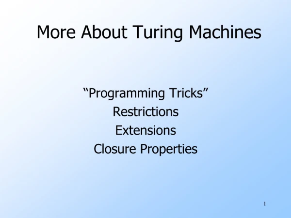
More About Turing Machines “Programming Tricks” Restrictions Extensions Closure Properties
Overview • At first, the TM doesn’t look very powerful. • Can it really do anything a computer can? • We’ll discuss “programming tricks” to convince you that it can simulate a real computer.
Overview – (2) • We need to study restrictions on the basic TM model (e.g., tape is infinite in only one direction). • Assuming a restricted form makes it easier to talk about simulating arbitrary TM’s. • That’s essential to exhibit a language that is not recursively enumerable.
Overview – (3) • We also need to study generalizations of the basic model. • Needed to argue there is no more powerful model of what it means to “compute.” • Example: A nondeterministic TM with 50 six-dimensional tapes is no more powerful than the basic model.
Programming Trick: Multiple Tracks • Think of tape symbols as vectors with k components. • Each component chosen from a finite alphabet. • Makes the tape appear to have k tracks. • Let input symbols be blank in all but one track.
Represents input symbol 0 Represents the blank Represents one symbol [X,Y,Z] Picture of Multiple Tracks q 0 X B B Y B B Z B
Programming Trick: Marking • A common use for an extra track is to mark certain positions. • Almost all cells hold B (blank) in this track, but several hold special symbols (marks) that allow the TM to find particular places on the tape.
Unmarked W and Z Marked Y Marking q B X B W Y Z
Programming Trick: Caching in the State • The state can also be a vector. • First component is the “control state.” • Other components hold data from a finite alphabet.
Example: Using These Tricks • This TM doesn’t do anything terribly useful; it copies its input w infinitely. • Control states: • q: Mark your position and remember the input symbol seen. • p: Run right, remembering the symbol and looking for a blank. Deposit symbol. • r: Run left, looking for the mark.
Example – (2) • States have the form [x, Y], where x is q, p, or r and Y is 0, 1, or B. • Only p uses 0 and 1. • Tape symbols have the form [U, V]. • U is either X (the “mark”) or B. • V is 0, 1 (the input symbols) or B. • [B, B] is the TM blank; [B, 0] and [B, 1] are the inputs.
The Transition Function • Convention: a and b each stand for “either 0 or 1.” • δ([q,B], [B,a]) = ([p,a], [X,a], R). • In state q, copy the input symbol under the head (i.e., a ) into the state. • Mark the position read. • Go to state p and move right.
Transition Function – (2) • δ([p,a], [B,b]) = ([p,a], [B,b], R). • In state p, search right, looking for a blank symbol (not just B in the mark track). • δ([p,a], [B,B]) = ([r,B], [B,a], L). • When you find a B, replace it by the symbol (a ) carried in the “cache.” • Go to state r and move left.
Transition Function – (3) • δ([r,B], [B,a]) = ([r,B], [B,a], L). • In state r, move left, looking for the mark. • δ([r,B], [X,a]) = ([q,B], [B,a], R). • When the mark is found, go to state q and move right. • But remove the mark from where it was. • q will place a new mark and the cycle repeats.
q B Simulation of the TM . . . B B B B . . . . . . 0 1 B B . . .
p 0 Simulation of the TM . . . X B B B . . . . . . 0 1 B B . . .
p 0 Simulation of the TM . . . X B B B . . . . . . 0 1 B B . . .
r B Simulation of the TM . . . X B B B . . . . . . 0 1 0 B . . .
r B Simulation of the TM . . . X B B B . . . . . . 0 1 0 B . . .
q B Simulation of the TM . . . B B B B . . . . . . 0 1 0 B . . .
p 1 Simulation of the TM . . . B X B B . . . . . . 0 1 0 B . . .
Semi-infinite Tape • We can assume the TM never moves left from the initial position of the head. • Let this position be 0; positions to the right are 1, 2, … and positions to the left are –1, –2, … • New TM has two tracks. • Top holds positions 0, 1, 2, … • Bottom holds a marker, positions –1, –2, …
0 1 2 3 . . . q You don’t need to do anything, because these are initially B. Put * here at the first move * -1 -2 -3 . . . U/L Simulating Infinite Tape by Semi-infinite Tape State remembers whether simulating upper or lower track. Reverse directions for lower track.
More Restrictions – Read in Text • Two stacks can simulate one tape. • One holds positions to the left of the head; the other holds positions to the right.
Extensions • More general than the standard TM. • But still only able to define the RE languages. • Multitape TM. • Nondeterministic TM. • Store for key-value pairs.
Multitape Turing Machines • Allow a TM to have k tapes for any fixed k. • Move of the TM depends on the state and the symbols under the head for each tape. • In one move, the TM can change state, write symbols under each head, and move each head independently.
Simulating k Tapes by One • Use 2k tracks. • Each tape of the k-tape machine is represented by a track. • The head position for each track is represented by a mark on an additional track.
Picture of Multitape Simulation q X head for tape 1 . . . A B C A C B . . . tape 1 X head for tape 2 . . . U V U U W V . . . tape 2
Nondeterministic TM’s • Allow the TM to have a choice of move at each step. • Each choice is a state-symbol-direction triple, as for the deterministic TM. • The TM accepts its input if any sequence of choices leads to an accepting state.
Simulating a NTM by a DTM • The DTM maintains on its tape a queue of ID’s of the NTM. • A second track is used to mark certain positions: • A mark for the ID at the head of the queue. • A mark to help copy the ID at the head and make a one-move change.
Front of queue Where you are copying IDk with a move Picture of the DTM Tape X Y ID0 # ID1 # … # IDk # IDk+1 … # IDn # New ID Rear of queue
Operation of the Simulating DTM • The DTM finds the ID at the current front of the queue. • It looks for the state in that ID so it can determine the moves permitted from that ID. • If there are m possible moves, it creates m new ID’s, one for each move, at the rear of the queue.
Operation of the DTM – (2) • The m new ID’s are created one at a time. • After all are created, the marker for the front of the queue is moved one ID toward the rear of the queue. • However, if a created ID has an accepting state, the DTM instead accepts and halts.
Sum of k+k2+…+kn Why the NTM -> DTM Construction Works • There is an upper bound, say k, on the number of choices of move of the NTM for any state/symbol combination. • Thus, any ID reachable from the initial ID by n moves of the NTM will be constructed by the DTM after constructing at most (kn+1-k)/(k-1)ID’s.
Why? – (2) • If the NTM accepts, it does so in some sequence of n choices of move. • Thus the ID with an accepting state will be constructed by the DTM in some large number of its own moves. • If the NTM does not accept, there is no way for the DTM to accept.
Taking Advantage of Extensions • We now have a really good situation. • When we discuss construction of particular TM’s that take other TM’s as input, we can assume the input TM is as simple as possible. • E.g., one, semi-infinite tape, deterministic. • But the simulating TM can have many tapes, be nondeterministic, etc.
Real Computers • Recall that, since a real computer has finite memory, it is in a sense weaker than a TM. • Imagine a computer with an infinite store for name-value pairs. • Generalizes an address space.
Simulating a Name-ValueStore by a TM • The TM uses one of several tapes to hold an arbitrarily large sequence of name-value pairs in the format #name*value#… • Mark, using a second track, the left end of the sequence. • A second tape can hold a name whose value we want to look up.
Lookup • Starting at the left end of the store, compare the lookup name with each name in the store. • When we find a match, take what follows between the * and the next # as the value.
Insertion • Suppose we want to insert name-value pair (n, v), or replace the current value associated with name n by v. • Perform lookup for name n. • If not found, add n*v# at the end of the store.
Insertion – (2) • If we find #n*v’#, we need to replace v’ by v. • If v is shorter than v’, you can leave blanks to fill out the replacement. • But if v is longer than v’, you need to make room.
Insertion – (3) • Use a third tape to copy everything from the first tape at or to the right of v’. • Mark the position of the * to the left of v’ before you do. • Copy from the third tape to the first, leaving enough room for v. • Write v where v’ was.
Closure Properties of Recursive and RE Languages • Both closed under union, concatenation, star, reversal, intersection • Recursive also closed under complementation.
Union • Let L1 = L(M1) and L2 = L(M2). • Assume M1 and M2 are single-semi-infinite-tape TM’s. • Construct 2-tape TM M to copy its input onto the second tape and simulate the two TM’s M1 and M2 each on one of the two tapes, “in parallel.”
Union – (2) • Recursive languages: If M1 and M2 are both algorithms, then M will always halt in both simulations. • Accept if either accepts. • RE languages: accept if either accepts, but you may find both TM’s run forever without halting or accepting.
Remember: = “halt without accepting Picture of Union/Recursive Accept M1 Reject OR Accept Input w M Accept M2 Reject AND Reject
Picture of Union/RE Accept M1 OR Accept Input w M Accept M2
Intersection/Recursive – Same Idea Accept M1 Reject AND Accept Input w M Accept M2 Reject OR Reject
Intersection/RE Accept M1 AND Accept Input w M Accept M2
Complement • Recursive languages: both TM’s will eventually halt. • Accept if M1 accepts and M2 does not. • Corollary: Recursive languages are closed under complementation. • RE Languages: can’t do it; M2 may never halt, so you can’t be sure input is in the difference.