Download
1 / 88
920 likes | 1.86k Views
Labor Supply, Demand & Unemployment. Mid-term Exam. Tuesday, October 12 th 9AM Lecture Theater E Semi-open Book (Bring 1 A4 size paper with handwritten notes)) Coverage. Lecture notes including this one. Hours per Worker 2005 www.ggdc.net. This section will follow.

E N D
Mid-term Exam • Tuesday, October 12th 9AM • Lecture Theater E • Semi-open Book (Bring 1 A4 size paper with handwritten notes)) • Coverage. Lecture notes including this one.
This section will follow • Branson, Chapter 6, 105-121 • Williamson, Chapter 4, 90-130 • Williamson, Chapter 15, 539-557 • Romer, Chapter 4, Section 4 & Chapter 9
Labor Demand • Output is a diminishing function of labor holding the capital stock constant. • The marginal product of labor is the slope of the production function. • The slope is diminishing as labor increases. We can map a function of this slope. • Firms will hire workers until the marginal benefit of hiring workers exceeds the marginal cost. To maximize profits, firms hire workers until the marginal product of labor equals the real wage.
Marginal Product of Labor = Slope of Production Function Q MPL2 MPL1 MPL L L0 L1 L2
Labor Demand Curve w0 w1 w2 MPL L L1 L0 L2
Labor Demand Curve • A mapping between the marginal product of labor and real wage is equivalent to the amount of labor demanded by firms. • To close out the model, we need a theory of labor supply. • Labor demand is based on the profit maximization of firms. We need a similar metric to measure the objective of workers.
Utility Function • When workers make a choice of how many hours to work, they make a trade-off between the goods they can buy with their wages and the leisure time they lose by working. • Workers will have preferences over a set of consumption-leisure choices. • An indifference curve is a set of leisure-combination choices over which the worker is indifferent.
Worker Preferences: More is Better • We assume workers prefer more to less. At any level of leisure, lst, it is always preferred to have more consumption of goods, Ct. • This implies that U0 is preferred to U1 which is preferred to U2.
The higher the indifference curve, the more it is preferred by workers. C U0 U1 U2 ls
Preference for Variety • Consumption and leisure have diminishing returns. • The slope of the indifference curve, MRS, is equal to the amount of consumption you would have to get in order to make you just as happy if you had to give up some leisure. • Along any indifference curve, the greater is lst the lower will be MRS
Diminishing Returns to leisure and Consumption. C -MRS1 U2 -MRS0 ls ls0 ls1
Goods are Normal • If overall income increases and relative prices remain the same, households will want to consume a greater amount of all goods. • If you won the lottery, you would probably would work less hard and consume more goods, so it is reasonable to assume that consumption and leisure are normal goods.
Utility Functions • Economists often act as if preferences over some choice set can be written as a mathematical function of the choices. • Conjecture a utility function which ranks the different choices giving a higher score to preferred choices. • For example, we might write a utility function in terms of consumption and leisure U(Ct,lst).
Utility Functions • More is better • Goods have diminishing returns.
Normal Goods • A simple way to insure that the utility function represents the preferences of a consumer for whom goods are normal is to let both goods enter in parallel ways.
Budget Constraint • Given the resources of the worker, they will have only a limited set of combinations of consumption and leisure which they will be able to choose. • Assume a limited set of time, TIME, available for workers which must be split between leisure and work, Nt.
Budget • Workers will have an income available for consumption equal to wages plus profits, Πt (net of investment) minus a poll tax Tt. • Given time constraints, we can write consumption as a negative function of leisure. The slope of this function is the real wage rate.
Budget Constraint. C w Π-T ls TIME
Optimal Consumption & Leisure: Geometry • We choose the most preferred consumption/leisure combo which gives the greatest utility subject to that combo being feasible. • Geometrically, this is where an indifference curve is tangent to the budget line. • The tangent indifference curve touches the budget line but does not cross, so it is by definition the top indifference curve that is part of the budget line.
Optimal Consumption Leisure C [C*,ls*] ls TIME
Optimal Consumption & Leisure:Intuition • The slope of the indifference curve is how much extra consumption you would need to get to make you just as well off to give up some leisure. • The slope of the budget line is the amount of extra consumption you can actually get if you give up some leisure • At any point, you would always willingly give up more leisure if the slope of indifference curve is less than the real wage. • You would also willingly give up consumption if the slope of the indifference curve was steeper than the real wage.
Optimal Consumption & Leisure: Intuition • At optimum, the slope of the indifference curve would be equal to the real wage. • At optimum, the marginal benefit of some extra leisure is equal to the marginal cost of leisure. The marginal cost of leisure is the real wage times the marginal value of the consumption that the real wage could by.
Optimal Consumption and Leisure: Calculus • Maximize U(Ct,lst) subject to the constraint that • Rewrite the utility function by inserting the constraint • Write the first order conditions as
Example • Log-log utility function • Objective Function • First Order Conditions
Elasticity of Substitution • For log,log utility, we can write the first order condition as • The real wage is the opportunity cost/price of leisure in terms of consumption. • A 1% increase in the relative price of leisure leads to a 1% increase relative demand for leisure. • Log,log utility is unit elasticity of substitution utility function.
Labor Supply Curve • The solution to the first order condition maps real wages, profit and tax income into an amount of labor • The labor supply curve is a mapping of the real wage into an optimal amount of labor provided by workers at a given amount of profit income and taxes.
Increase in Lump-sum Income • If leisure & consumption are normal goods, an increase in profit or a cut in taxes will increase the amount of leisure that is desired. This will in turn cut the labor supply. • Income Effect: At a constant wage rate, an increase in income would increase consumption. This would reduce the marginal value of any wage income earned because consumption has diminishing returns. Thus, the marginal cost of leisure would drop inducing workers to take more leisure.
Effect of Wages on Labor Supply • There are two channels through which an a change in the wage rate affects the marginal cost of leisure. • Substitution Effect: An increase in the wage rate directly increases the cost of not working because it increases the pay-off to each hour worked. This will tend to make the worker substitute additional income for leisure.
Income Effect 2. Income Effect: An increase in wages increases income & consumption, decreases the marginal utility of consumption, and decreases the welfare value of wages. The income effect will tend to make the worker choose to enjoy more leisure time.
Income vs. Substitution Effect • In theory, there are no clear assumptions about preferences that would make us think that either the income or the substitution effect would be stronger. • In theory, either effect could be stronger and an increase in wages could have either effect.
Wages Rise C Income Effect Pure Substitution Effect [C*,ls*] ls TIME
Example • If there were no profit income and no taxes in the log-log case, then the income and substitution effects would exactly cancel out and labor supply would not depend on real wages. • Given positive profits, a rise in the real wage relative to profits will increase the optimal labor choice.
Upward Sloping Supply Curve & Equilibrium w0 LS w* LD L L*
Capital or Technology Increase/ Labor Demand Curve Shifts Out/ Equilibrium Wages and Employment Increases w0 LS w** w* LS LD’ LD L L* L**
Profit or Tax Increase/ Labor Supply Shifts Out / Equilibrium Wages Fall and Employment Increases w0 LS LS’ w* w*** LD’ LD L L* L***
Taxes • Raising income tax rates has counter-veiling impacts on supply. • Lump sum taxes/poll taxes have a positive impact on labor suppy.
Is an Upward Sloping Labor Supply Consistent with Long Term? • Over the very long-term, productivity and real wages have risen by a large amount and labor supply per person has been falling, if anything. • Over the long-run, non-labor income should be rising along with real wages. Thus, this income effect may be driving labor down.
Upward Sloping Labor Supply in the Short Run • The level of consumption depends on the level of lifetime income. • A temporary rise in real wages will not have a strong effect of lifetime income. • Thus, a temporary increase in real wages will have a strong substitution effect and a weak income effect.
Unemployment Rate • The population is split into three categories: • (NLt) Not in the Labor Force: those people who do not have jobs and are not actively seeking employment. • (Et) Employed, those people who currently have jobs. • (Ut) Unemployed, those people seeking jobs.
The labor force participation rate is the share of the population which are employed or unemployed. • The unemployment rate is that share of the labor force which is unemployed.
Types of Employment • Frictional – Unemployment that results from the standard dynamic nature of the labor market. When people change jobs, there is frequently some period when they are looking for work. • Structural – Unemployment that results from some big change in the economy caused by new trade competition or new technology. • Cyclical – Unemployment associated with the business cycle. We will concentrate on type 1 in this section.
Data • The Bureau of Labor Statistics of the USA Department of Labor maintains a large database of international unemployment rates, wage rates, inflation rates, and productivity levels (in addition to extensive US labor market and inflation measures). • The web-site http://www.bls.gov