Download

1 / 45
530 likes | 972 Views
Hamiltonian Cycles. Vesal Hakami October 30, 2010. Brief History Basic Definitions, Initiatives, Sufficient Conditions, A Backtracking Algorithm Chiba & Nishezeki ’s Linear Implementation for Internally 4-Connected Plane ( I4CP ) Graphs ( Journal of Algorithms , 1989 – Elsevier).

E N D
Hamiltonian Cycles VesalHakami October 30, 2010
Brief History • Basic Definitions, Initiatives, Sufficient Conditions, A Backtracking Algorithm • Chiba & Nishezeki’s Linear Implementation for Internally 4-Connected Plane (I4CP) Graphs (Journal of Algorithms, 1989 – Elsevier)
Icosian game invented by Sir. William Rowan Hamilton (1805–1865) in 1857 and sold to a London game dealer in 1859 for 25 pounds. • Game Description: The corners of a regular dodecahedron are labeled with the names of cities; the task is to find a circular tour along the edges of the dodecahedron visiting each city exactly once. • Solution Model: Hamiltonian cycle; i.e. look for a cycle in the corresponding dodecahedral graph which contains each vertex exactly once. The Platonic Solid used in Icosiangame; the corresponding Hamiltonian cycle is designated by darkened edges.
Hamiltonian Cycle: If G = (V, E) is a graph or multi-graph with |V|>=3, we say that G has a Hamiltonian cycle if there is a cycle in G that contains every vertex in V. • Hamiltonian Path: A Hamiltonian path is a path (and not a cycle) in G that contains each vertex. It is possible, however, for a graph to have a Hamiltonian path without having a Hamiltonian cycle. Hamiltonian path Hamiltonian cycle * Necessary and Sufficient Conditions for Hamiltonian based on Linear Diophantine Equation Systems with Cycle Vector, 2009 3rd Intl. Conf. on Genetic and Evolutionary Computing.
Does G contain a Hamiltonian path? • Starting from vertex a, alternatively label each vertex and its adjacents with x’s and y’s. If G is to have a Hamiltonian path, there must be an alternating sequence of five x's and five y's. • Recall: A graph G = (V, E) is bipartite iff it contains no cycle of odd length. x-yvertex labeling 4 x’s and 5 y’s No Hamiltonian path G (no cycle of odd length) G is, in fact, a bipartite graph
Theorem. A complete digraph (called a tournament)- in which for each distinct pair x, y of vertices, exactly one of the edges (x, y) or (y, x) is in - always contains a (directed) Hamiltonian path. • Proof: • Let m 2 with Pm a path containing the m-1 edges (v1, v2), (v2, v3), .... (vm-1, vm). • if m = n, we're finished. • If not, • let v be a vertex that does not appear in Pm. • If (v, v1) is an edge in , we can extend Pm by adjoining this edge. • If not, • (v1, v) must be an edge. • Suppose that (v, v2) is in the graph. • We have the larger path: (v1, v), (v, v2), (v2, v3), ..., (vm-1, vm). • If (v, v2) is not an edge in , then (v2, v) must be. • Continue this process; there are only two possibilities: • (a) For some 1km-1, the edges (vk, v), (v, vk+1) are in and we replace (vk, vk+1) with this pair of edges. • (b) (vm, v) is in and we add this edge to Pm. • Either case results in a path Pm+1that includes m+1 vertices and has m edges. • Repeat this process until we have a path Pn on n vertices.
Theorem. Let G= (V, E) be a loop-free graph with |V|= n 2. If deg(x) + deg(y) n - 1 for all x, yV, xy, then G has a Hamiltonian path. • Proof. • I) Connectivity(Proof by Contradiction): G consists of two components C1(|C1| = n1) and C2 (|C2| = n2). Let xC1 and yC2. Obviously, deg(x)n1 - 1 and deg(y) n2 - 1; that is, deg(x) + deg(y) (n1 + n2) – 2 n - 2, contradicting the condition given in the theorem; thus, G is connected. • II) Hamiltonian path construction: • For m2, let Pm be the path {v1, v2}, {v2, v3}, ... , {vm-1, vm} of length m - 1. • If v1 is adjacent to any vertex v other than v2, v3, ..., vm, we add the edge {v, v1} to Pm to get Pm+1. • The same procedure is carried out if vm is adjacent to a vertex other than v1, v2, ..., vm-1. • If we are able to enlarge Pm to Pn in this way, we get a Hamiltonian path.
Otherwise, • Pm: {v1, v2}, ..., {vm-1, vm} has v1 and vm adjacent only to vertices in Pmand m < n. • Now, we claim that G has a cycle on these vertices: • If v1 and vm are adjacent, then the cycle is {v1, v2}, {v2, v3}, ..., {vm-1, vm}, {vm, v1}. • Otherwise, • v1is adjacent to a subset S of the vertices in {v2, v3, ..., vm-1}. • If there is a vertex vtS such that vm is adjacent to vt-1, then we can get the cycle by adding {v1, vt}, {vt-1, vm} to Pm and deleting {vt-1, vt}, as shown in Fig. (a). Fig. (a) • If not, • Let |S| = k < m - 1. • Then, deg(v1) = k and deg(vm) (m - 1) - k • Contradiction! deg(v1) + deg(vm) m - 1 < n - 1. • Hence, there is a cycle connecting v1, v2, ..., vm.
Corollary. • Now, consider a vertex vV that is not found on this cycle. • G is connected, so there is a path from v to a first vertex vr in the cycle, as shown in Fig. (b). Fig. (b) • Removing the edge {vr-1, vr} (or {v1, vt} if r = t), we get the path (longer than the original Pm) show in Fig. (c). • Repeating this whole process for the path in Fig. (c), we continue to increase the length until it includes every vertex of G. Fig. (c) The loop-free graph G = (v, E) with |V| 2 has a Hamiltonian path if deg(v) (n - 1)/2 for all vV.
Theorem. Let G= (V, E) be a loop-free graph with |V|= n3. If deg(x) + deg(y) nfor all x, yV, xy, then G has a Hamiltonian cycle. • Proof. • Assume that G does not contain a Hamiltonian cycle. • We add edges to G until we arrive at a sub-graph H of Kn, where H has no Hamiltonian cycle, but, for any edge e (of Kn) not in H, H + e does have a Hamiltonian cycle. • Since HKn, there are vertices a, bV, where {a, b} is not an edge of H but H + {a, b} has a Hamiltonian cycle C. • The graph H has no such cycle, so the edge {a, b} is a part of cycle C. • The vertices of H (and G) on cycle C are as follows:
For each 3 in, if the edge {b, vi} is in the graph H, • then we claim that the edge {a, vi-1} cannot be an edge of H. • If both of these edges are in H, for some 3in, • we get the Hamiltonian cycle: • for the graph H (which has no Hamiltonian cycle). • Therefore, for each 3 in, at most one of the edges {b, vi}, {a, vi-1} is in H. • Consequently, • Since for all vV, , so we have nonadjacent (in G) vertices a, b, where CONTRADICTION!
Corollary I.If G = (V, E) is a loop-free undirected graph with |V| = n 3, and if deg(v) n/2 for all vV, then G has a Hamiltonian cycle. • Corollary II. If G = (V, E) is a loop-free undirected graph with |V| = n 3, and if , then G has a Hamiltonian cycle. • Proof. • Let a, bV, where {a, b} is not in E. [Since a, b are nonadjacent, we want to show that deg(a) + deg(b) >= n.] • Remove the vertices a and b together with all edges incident on them from the graph G. • Let H = (V', E') denote the resulting sub-graph. • |E| = |E'| + deg(a) + deg(b) because {a, b} is not in E.
Since |V'| = n - 2, H is a sub-graph of the complete graph Kn-2, so • Consequently, • and we find that:
State space tree: • The initial node in level 0 • All the remaining n-1 nodes in levels 1, 2, …, n-1 • The number of state space tree nodes: • Promising nodes’ characterization: • The ith node on the path must be adjacent to (i-1)th node • (n-1)th node must be adjacent to node 1 (initial node) • The ith node cannot be one of the first i-1 nodes • Inputs: • A positive integer n (Number of vertices) • An undirected graph G with n vertices and with adjacency matrix denoted by the 2D array W • Output: • The Hamiltonian cycle denoted by the linear array vindex • vindex[i] is the index of the ith node on the cycle. • The Index of the initial node is located in vindex [0].
High level call: • vindex[0] = 1; • hamiltonian(0); voidpromising (index i) { index j; boolswitch; if ( i == n – 1 && ! W[vindex[n – 1]] [vindex[0]]) // First vertex must switch = false; // be adjacent to else if (i > 0 && ! W[vindex[i -1]] [vindex[i]]) // last. ith vertex switch = false; // must be adjacent else { // to (i – 1)th. switch = true; j = 1; while (j < i && switch) { // Check if vertex is if (vindex[i] == vindex[j]) // already selected. switch = false; j++; } } returnswitch; } • voidhamiltonian (index i) • { index j; if (promising(i)) if (i == n – 1) cout << vindex[0] through vindex[n – 1]; else • for (j = 2; j <= n; j++) // Try all vertices • { // as next one. vindex[i + 1] = j; hamiltonian(i+1); } • }
The Hamiltonian cycle problem is NP-complete even for 3-connected planar graphs. • Tutteproved that a 4-connected planar (4CP) graph necessarily contains a Hamiltonian cycle and that It can be found in polynomial time. • Prior art for 4CP graphs: • An O(n3) algorithm • A linear algorithm for 4-connected “maximal” planar graphs • Objective • A linear algorithm for finding a Hamiltonian cycle in general 4CP graphs
Solution methodology • Divide & Conquer with inductive argument: • Decompose a graph into several small sub-graphs, then find Hamiltonian cycles in sub-graphs by applying the inductive hypothesis to them, and finally combine the Hamiltonian cycles into a Hamiltonian cycle of the whole graph. • Since the decomposed graphs are not always edge-disjoint, it was non-trivial to verify even the polynomial bounded-ness of the algorithm. • Key idea: • Avoid the decomposition into non-disjoint sub-graphs.
Cut-vertex: a vertex whose deletion increases the number of components. • Separation pair: a separation pair of a 2-connected graph G is two vertices whose deletion disconnects G. • Splitting: Dividing a graph G into two split graphsG1 and G2. • Merging: the inverse of splitting • Virtualedge: The edge {x, y} in G1 or G2whether it originally exists in G1 and G2 or is newly added to G1 and G2. • Separation triple: a separating set of three vertices. • 4-connected graph: a 3-connected graph with no separation triples. • Block: A block of G is a maximal 2-connected sub-graph of G.
Lemma. Let G be a 2-connected plane graph with the outer facial cycleZ. Let s and e = (a, b) be a vertex and an edge, both on Z, and let t be any vertex of G distinct from s. Then G has a path P(called a Tuttepath) going from s to t through esuch that • (i) each component of G - P is adjacent to at most three vertices of P, and • (ii) each component of G - P is adjacent to at most two vertices of P if it contains an edge of Z. Remark I. The above lemma implies that a 4-connected planar graph G has a Hamiltonian cycle.
Remark II. Let G be a 4-connected and P be a s, t- Tutte path in G. Suppose H is a (G - P)-component then, since G is 4-connected, H must have 4 vertices of attachment in P which is a contradiction because P is a Tutte path. • Remark III. In a 4-connected planar graph G: Let sand t be two adjacent vertices on Z and let e (s, t) be an edge on Z, then the path P joining s and t through e, assured by the Lemma, must be a Hamiltonian path of G, so P + (s, t) must be a Hamiltonian cycle of G. Thus an algorithm for finding the s-t path Pimmediately yields an algorithm for finding a Hamiltonian cycle. • Decomposition strategy • The original graph G is 4-connected. • The sub-graphs into which G is decomposed are no longer 4-connected. • They inherit the “internally 4-connected (I4C)” property.
The I4C property • Intuitively, a graph is internally 4-connected if it contains no separation pair or triple in the interior. • Formal definition: Let G be a 2-connected plane graph with outer facial cycle Z. Let s and tbe two distinct vertices on Z, and let e = (a, b) be an arbitrary edge on Zsuch that e (s, t). ta , b and vertices s, a, b and t appear clockwise on Zin this order. (Fig. (a).) • Possibly s = a as illustrated in Fig. (b). Let r be the vertex on Z counterclockwise next to s, and let f = (r, s) be the edge joining r and s.
A plane 2-connected graph G is internally 4-connected with respect to (s, t, e) if G satisfies the following two conditions: • If {x, y} is a separation pair, then • every component of G - {x, y} contains at least one vertex of Z • each of the three paths Psa, Pbt and Ptscontains at most one of xand y. (b) If {x, y, z} is a separation triple, then every component of G - {x, y, z} contains at least one vertex of Z. (c), (d) and (e) violate conditions in (a). (f) violates condition (b).
Vertical separation pair: a separation pair {x, y} is called vertical if either xPsa- s and yPbr or x = s and yPbt– t. • Type I Reduction: G is decomposed into two sub-graphs w.r.t. a vertical separation pair. • {y’, z’} is a horizontalseparation pair.
Let G be an I4CP graph having no vertical separation pair, then G is decomposed into several sub-graphs, called , , and. (If S = a, G is decomposed into and.) G
: the block of G – Psa which contains t. is cross-hatched.) • must entirely contain Pbr, otherwise G would contain a vertical separation pair. • Repeat splitting of at every separation pair such that one of the two split graphs entirely contains Pbr. • The component containing Pbr is called Gb, while each of the others is called where g = (x, y) is a virtual edge contained in the component.
maximal sub-graph of G – which can be separated from at each cut-vertex u. • the sub-graph of G induced by the vertices of and the vertices on Psawhich are adjacent to . • Let x (resp. y) be the vertex of which is nearest to s (resp. a) along . Add a new edge e’ = (u, y) to if it does not exist, and let be the resulting graph.
: schematically, is a graph formed by merging with all the and drawn above . • Constructively, is defined as: • := ; • while has a virtual edge g’g, iterate to merge into ; • for each cut-vertex u (x, y) of G – Psa contained in merge to ; • Construct the sub-graph of G induced by the vertices of together with the vertices of Psa adjacent to , and redefine as the sub-graph; • - x – y.
Lemma. Let G be an I4CP graph containing no vertical separation pair. Then, all the decomposed graphs , andare I4C w.r.t. (s’ , t’ , e’) if s’ , t’ , e’ are defined as follows: • - Case • s’ = b • t’= t • e’ = • if tr • the edge clockwise incident to r on the outer facial cycle of Gb. • If t = r • the edge counterclockwise incident to b.
Case s’ = y t’ = x e’ = the edge counterclockwise incident to y on the outer facial cycle of . • Case s’ = u t’ = x e’ = (u, y). • Case s’ = w t’ = v e’ = if w’ v’ an arbitrary edge on outer path Pw’v’. If w’ v’ an arbitrary edge on Pwv incident to w’ (= v’).
Proof. We verify only the case. Suppose is not I4C w.r.t. (s’ , t’ , e’). Then, must have one of the following three: • a cut-vertex vc. • A separation pair {vp1, vp2} such that both vp1 and vp2 are contained in path Pwa’ or Pbv’; and • a separation triple {vt1, vt2, vt3} for which one of the components of - {vt1, vt2, vt3} contains no vertex of the outer facial cycle Z’ of • In either case, G would contain a separation triple {vc, x, y}, {vp1, vp2, vx}, {vp1, vp2, y}, or {vt1, vt2, vt3} such that the deletion of the triple from G produces a component containing no vertex of Z. This contradicts the I4C-ness of G. G
Lemma. Let Gbe a plane graph having an outer facial cycle Z. Let sand t be two distinct vertices on Z and let e((s, t) ) be an edge on Z . If Gis I4C w.r.t. (s, t, e), then G has a Hamiltonian path P(G, s, t, e) which connects s and t and contains e. Moreover, if G has no vertical separation pair, then P(G, s, t, e) does not contain edge f = (s, r). • Proof. The proof is by induction on the number nof vertices of a graph G. If n= 3, the claim is clearly true, so we assume that n> 3. There are two cases to consider. • There exists a vertical separation pair {x, y} • G has no vertical separation pairs.
Case 1: There exists a vertical separation pair {x, y}. • Among all vertical separation pairs of G, we choose {x, y} such that Grhas the smallest number of vertices. We call such a separation pair the rightmostseparation pair. • Consider the case tGI* as shown in Fig. • Let e’ = (x, y) be a virtual edge. • Clearly, Glis I4C w.r.t. (s, t, e’), while Gr is I4C w.r.t. (x, y, e) (or w.r.t. (y, x, e) if y = b). • By the inductive hypothesis, Glhas a Hamiltonian path P(Gl, s, t, e’) and Grhas P(Gr, x, y, e). • G has a Hamiltonian path: • P(G , s, t, e) = P(Gl , s, t, e’) + P(Gr, x, y, e) – e’ • or P(Gl , s, t, e’) + P(Gr , y, x, e) – e’ • * The case tGI is handled with a similar understanding.
Case 2: G has no vertical separation pair. • By the inductive hypothesis, all the decomposed graphs , andhave Hamiltonian paths. From them, a Hamiltonian path P(G, s, t, e) of G can be constructed as follows (Note that edge f = (s, r) is never included in path P): First set P to Psb+ P(Gb, b, t, e’). While there is a virtual edge g = (x, y) in Gb If gP, then P : = P – g + P( , y, x, e’). (replace g of P by a H-path of ) Merge into Gb ; If gp, then Construct , and set P := P– Pvw+ P( , w, v, e’), Delete g from Gb . For each u of the cut-vertices of G – Psa contained in Gb Set P := P–Pxy+ P( , u, x, (u, y))- (u, y).
G , ,
In the previous slide, • The path passes through the virtual edge (1, 7), so a Hamiltonian path of is determined. • The path passes through the virtual edges (1, 3) and (5, 7) but not (3, 5), so the Hamiltonian paths of , and are determined. • S- t Hamiltonian path
Time Complexity Analysis procedureHPATH(G, s, t , e); begin ifG contains exactly three vertices then{Gis a triangle} return a (trivial) Hamiltonian path P(G, s, t, e); else if G has a vertical separation pair thenType I reduction elseType II reduction end; • Lemma. There are at most n-3 reductions during one execution of algorithm HPATH. • Theorem. The algorithm HPATH spends at most O(n2) time.
Proof. • r: the number of reductions occurred during one execution of HPATH. • d(i), 1 ir: the number of small graphs into which a graph is decomposed at the ith reduction; i.e. d(i) is the number of the recursive calls which occurred at the reduction. 2 if the ith reduction is of Type I d(i) = 1 if the ith reduction is of Type II and none of ,is produced. • r': the number of reductions with d = 1 • t: the number of final triangles
Upper bound on the number of reductions in the recursive call tree: • Internal nodes Reductions • Children of internal nodes Recursive calls at the reduction • LeavesFinal triangles • The tree has: • t leaves • r internal nodes (r' of which have out-degree 1) • Recall:The number of internal nodes in a binary tree is one less than the number of leaves. • The recursive tree has at most t - 1 internal nodes of out-degree 2 or more; thus, we have: rt – 1 + r’ (1)
Upper bound for the total length of paths found in triangles: • A Type I reduction increases by one the total length of paths which will be found in the two reduced graphs. • In general, the ith reduction increases by d(i) – 1 the total length of paths which will be found in the d(i) reduced graphs. • Conversely, if d(i) = 1, then the length of a path which will be found in the reduced graph decreases by at least one. • HPATH initially wishes to find a Hamiltonian path of length n – 1. Therefore, the upper bound for the total length of paths found in triangles is: = (2)
The lengths of the Hamiltonian paths found in the final triangles total 2t, we have: • that is, (3) • Combining (1) with (3), we get the claimed bound on r: r