Quantifying uncertainty in volcanic ash forecasts
240 likes | 255 Views
Learn how to improve confidence in volcanic ash forecasts by quantifying uncertainty using emulators to explore parameter spaces efficiently. Prioritize variables for operational ensembles and build trust in spatial forecasts.

Quantifying uncertainty in volcanic ash forecasts
E N D
Presentation Transcript
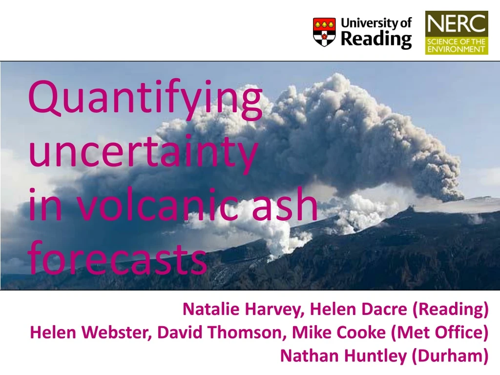
Quantifying uncertainty in volcanic ash forecasts Natalie Harvey, Helen Dacre (Reading) Helen Webster, David Thomson, Mike Cooke (Met Office) Nathan Huntley (Durham)
Improving confidencein volcanic ash forecasts Natalie Harvey, Helen Dacre (Reading) Helen Webster, David Thomson, Mike Cooke (Met Office) Nathan Huntley (Durham)
Probabilistic ForecastExample: 1200 14 May 2010 Medium contamination (2x10⁻³ g/m3)
Sources of uncertainty Missing processes Imperfect model
With this emulator, we can explore the parameter space much faster, and furthermore identify plausible and implausible regions (for instance through history matching). Early investigations suggest that the average concentration over a particular region and time can be used to build useful emulators. Quantifying uncertaintyEmulation 3 variables 2 variables 1 variable
With this emulator, we can explore the parameter space much faster, and furthermore identify plausible and implausible regions (for instance through history matching). Early investigations suggest that the average concentration over a particular region and time can be used to build useful emulators. Quantifying uncertaintyEmulation More than 3 variables? 3 variables 2 variables 1 variable
With this emulator, we can explore the parameter space much faster, and furthermore identify plausible and implausible regions (for instance through history matching). Early investigations suggest that the average concentration over a particular region and time can be used to build useful emulators. Quantifying uncertaintyEmulation • Dispersion model • Complex – over 25 different parameters • Runs slowly • Can’t easily understand interactions • Emulator • Simple approximation of complex model • Quickly evaluated over large range of parameter space • Identify parameters that contribute most to the uncertainty in the output and interactions between them 1. Variable 3 2. Variable 7 3. Variable 1 4. Variable 22 ….. Statistics happens here! Statistics happens here!
Quantifying uncertaintyExample: 14 May 2010 • 500 NAME runs • 15 parameters varied (all at the same time) • Parameter ranges determined by experts in the field
Quantifying uncertaintyExample: 14 May 2010 • Emulate average ash column loading in 81 pre-determined regions (2/3 per hour) Satellite “Best guess” model
Quantifying uncertaintyMost important parameters • This information can be used to inform future research and measurement campaigns. • Prioritise variables (and their ranges) to perturb for a small operational ensemble plume height and mass eruption rate Free tropospheric turbulence Precipitation level required for wet deposition Particle size distribution
What is a good spatial forecast? Example: 14 May 2010 Model Visible satellite RGB satellite Ash loadings IASI ash index
What is a good spatial forecast?Spatial comparison Problem: Model output is more spatially coherent with a wide range of concentration values compared to the satellite. This is due to the satellite having a detection limit. Answer: Match the number of model pixels to the number of satellite pixels before performing comparison. Choose pixels with highest levels of ash Column loading (µg/m2)
What is a good spatial forecast?Spatial comparison • Look in the neighbouring grid boxes and compares the fraction containing ash • Increase neighbourhood size to get measure of “useful” skill or scale at which we “trust” the forecast Model Obs Model Obs
What is a good spatial forecast? Spatial comparison Satellite Model Scale 200 km 5 times grid scale 40 km grid scale Harvey & Dacre (2015)
Probabilistic Forecast?Many realisations Different information about the volcano Different input meteorology Different model parameters Different models
Probabilistic Forecast?Ash concentration threshold Low contamination (2x10⁻⁴ g/m3) Medium contamination (2x10⁻³ g/m3)
Probabilistic Forecast?Probability threshold Low contamination (2x10⁻⁴ g/m3) One model run
Probabilistic Forecast?Region of interest Source: EUROCONTROL
Probabilistic Forecast?Region of interest Fraction of FIR with ash Maximum fraction in FIR Mean fraction in FIR
Probabilistic Forecast?Along flight path High contamination One model realisation Medium contamination Low contamination Ten model realisations
Probabilistic Forecast?Impact models? Impact model
Improving confidence in volcanic ash forecasts • Emulation can be used to find the parameters that contribute most to the uncertainty in model output • Inform research priorities • Prioritise variables to perturb for a small operational ensemble • Now have a metric which can be used to determine the scale over which a model can be trusted and can be applied to probabilistic forecasts • What is the most useful way to convey probabilistic information to decision makers?