Download
1 / 50
500 likes | 547 Views
Delve into the realm of quantum computers, exploring their potential, feasibility, and the interplay of noise and computational power at different scales. Discover the fundamental differences between classical and quantum computing.

E N D
The Quantum Computer Puzzle Gil Kalai Einstein Institute of Mathematics Hebrew University of Jerusalem Distinguished Lecture Series Department of Mathematics Indiana University Bloomington Fall 2016
Plan of the talks • Lecture I: The quantum computer puzzle • Lecture II: Elections – noise stability, noise sensitivity and the anomaly of majority. • Lecture III: What can we learn from the failure of quantum computers.
Quantum computers and quantum supremacy Quantum computers are hypothetical devices, based on quantum physics, which would enable us to perform certain computations hundreds of orders of magnitude faster than digital computers. This feature is coined “quantum supremacy”, and a famous example is Peter Shor’s quantum algorithm for factoring. One aspect or another of quantum supremacy might be seen by experiments in the near future: by implementing quantum error-correction or by systems of non-interacting bosons or by exotic new phases of matter called anyons or by quantum annealing, or in various other ways. Are quantum computers feasible? This is an important clear-cut scientific/technological question.
A summary of my view (1) Understanding quantum computers in the presence of noise requires consideration of behavior at different scales. In the small scale, standard models of noise from the mid-90s are suitable, and quantum evolutions and states described by them manifest a very low-level computational power. This represents a joint work with Guy Kindler (2014) and is based on my 1999 work with ItaiBenjamini and Oded Schramm.
A summary of my view (2) This small-scale behavior has far-reaching consequences for the behavior of noisy quantum systems at larger scales. On the one hand, it does not allow reaching the starting points for quantum fault tolerance and quantum supremacy, making them both impossible at all scales. On the other hand, it leads to novel implicit ways for modeling noise at larger scales and to various predictions on the behavior of noisy quantum systems. This represents my earlier papers from 1996-2011, and it was the subject of an Internet debate with Aram Harrow.
A question by Itai Benjamini (May, 2016) Will your view be proved wrong between now and the lecture? (Answer: Probably not, but it is widely expected that my view will come to test in a couple of years.) Other FAQ: Does your stance express concerns regarding the technology or does it amount to some basic law of nature? (Answer: Probably it’s quite basic) Does a failure of quantum computers accounts for breakdowm of quantum mechanics? (Answer: NO)
What is computation? The basic memory component in classical computing is a bit, which can be in two states, “0” or “1”. A computer (or circuit) has 𝑛 bits, and it can perform certain logical operations on them. The NOT gate, acting on a single bit, and the AND gate, acting on two bits, suffice for universal classical computing. Classical circuits equipped with random bits lead to randomized algorithms, which are both practically useful and theoretically important
What is a qubit? Quantum computers (or circuits) allow the creation of probability distributions that are well beyond the reach of classical computers with access to random bits. A qubit is a piece of quantum memory. The state of a qubit can be described by a unit vector in a 2-dimensional complex Hilbert space H. For example, a basis for 𝐻 can correspond to two energy levels of the hydrogen atom or to horizontal and vertical polarizations of a photon. Quantum mechanics allows the qubit to be in a superposition of the basis vectors, described by an arbitrary unit vector in 𝐻.
What is a quantum computer? The memory of a quantum computer (quantum circuit) consists of nqubits. The state of the computer is a unit vector in the tensor product of all the 2-dimensional Hilbert spaces corresponding to the qubits. We can put one or two qubits through gates representing unitary transformations acting on the corresponding two- or four-dimensional Hilbert spaces, and as for classical computers, there is a small list of gates sufficient for universal quantum computing. Each step in the computation process consists of applying a unitary transformation on the large 2𝑛 -dimensional Hilbert space, namely, applying a gate on one or two qubits, tensored with the identity transformation on all other qubits.
Measuring Measuring the state of a single qubit leads to a random bit described by a probability distribution on ‘0’ and ‘1’. At the end of the computation process, the state of the entire computer can be measured, giving a probability distribution on 0–1 vectors of length 𝑛.
Efficient computation and Computational complexity • Computational complexity is the theory of efficient computations, where “efficient” is an asymptotic notion referring to situations where the number of computation steps (“time”) is at most a polynomial in the number of input bits • The complexity class P is the class of algorithms that can be performed using a polynomial number of steps in the size of the input. • The complexity class NP refers to nondeterministic polynomial time. Roughly speaking, it refers to questions where we can provably perform the task in a polynomial number of operations in the input size, if we are given a certain polynomial-size “hint” of the solution. • P and NP are two of the lowest computational complexity classes in the polynomial hierarchy PH, which is a countable sequence of such classes. • Factoring is in NP, but it is unlikely that it is NP-complete. Shor’s famous algorithm shows that quantum computers can factor 𝑛-digit integers efficiently—in ∼ 𝑛2 steps! • Our understanding of the computational complexity world depends on a whole array of conjectures: NP ≠ P is the most famous one.
Drawing computational complexity insights on small systems Computational complexity insights, while asymptotic, strongly apply to finite and small algorithmic tasks. Paul Erdős famously claimed that finding the value of the Ramsey number 𝑅(6, 6) is well beyond mankind’s ability. This statement is supported by computational complexity insights that consider the difficulty of computations of R(n,n) as 𝑛 → ∞, while not directly implied by them.
Ramsey numbers The Ramsey number R(n,n) is the smallest integer m so that in every coloring of the edges of a complete graph Km with two colors, there is a monochromatic complete graph on n colors. “Paul Erdős asks us to imagine an alien force, vastly more powerful than us, landing on Earth and demanding the value of R(5, 5) or they will destroy our planet. In that case, he claims, we should marshal all our computers and all our mathematicians and attempt to find the value. But suppose, instead, that they ask for R(6, 6). In that case, he believes, we should attempt to destroy the alien force.”
Noise The main concern from the start regarding the feasibility of quantum computers was that quantum systems are inherently noisy; we cannot accurately control them, and we cannot accurately describe them. To overcome this difficulty, a theory of quantum fault-tolerance based on quantum error-correction was developed. Noise refers to the general effect of neglecting degrees of freedom. The study of noise is relevant not only to controlled quantum systems but to many other aspects of quantum physics.
The Optimistic Hypothesis Optimistic Hypothesis: The effort required to obtain a bounded error level for universal quantum circuits increases moderately with the number of qubits. It is therefore possible to realize universal quantum circuits with a small bounded error level regardless of the number of qubits. Thus, large-scale fault-tolerant quantum computers are possible.
The Pessimistic Hypothesis Pessimistic Hypothesis: The effort required to obtain a bounded error level for any implementation of universal quantum circuits increases (at least) exponentially with the number of qubits. Therefore, for every realization of universal quantum circuits the error rate scales up (at least) linearly with the number of qubits These difficulties will be demonstrated for small quantum systems with handful of qubits. Thus, quantum computers are not possible.
The optimistic and pessimistic hypotheses The gap between the two points of view is large. It could be tested in the next few years. The two hypotheses are based on the same basic noise model for noisy quantum circuits. Both hypotheses are compatible with quantum mechanics. The pessimistic hypothesis suggests that quantum supremacy is an artifact of incomplete account for “locality” in the quantum circuit model.
Noise sensitivity and noise stability A Boolean function f(x1,x2,…,xn) is a function from {-1,1}nto {-1,1}. A family of Boolean functions is balanced if the probability that f=1 is (uniformly) bounded away from 0 and from 1. A Boolean function is monotone if changing the value of a variable from -1 to 1 cannot change the value of f from 1 to -1. t-noise refers to switching the value of each variable with probability t independently. (t is a small real number.) A class of balanced Boolean function is (uniformly) noise stable if for every t > 0 The correlation between f(x) and f(Nt(x)) is bounded away from 0. .
Noise sensitivity and noise stability Theorem (Benjamini, Kalai, Schramm 99): Noise stability is equivalent to low-degree Fourier-Walsh coefficients Theorem (Benjamini, Kalai, Schramm 99): A class of monotone balanced Boolean functions is noise stable if and only if it has a uniformly positive correlation with a weighted majority functions.
Fermions and bosons Fermions – particles characterized by the Fermi-Dirac statistics; examples: electrons, quarks, leptons, protons and neutrons. Bosons – particles characterized by the Bose-Einstein statistics; examples: photons, gluons, the Higgs boson. Fermionic statistics – the state of several indistinguishable non interacting fermions is described by determinants. Bosonic statistics – the state of several indistinguishable non interacting fermions is described by permanents.
BosonSampling Manipulation of nnoninteracting bosons will allow sampling n by nsubmatrices of a prescribed n by m matrix according to the values of the permanent. BosonSampling was introduced by Troyansky and Tishby in 1996 and was intensively studied by Aaronson and Arkhipov, who offered it as a quick path for experimentally showing that quantum supremacy is a real phenomenon.
Sampling via free bosons Consider the input matrix The output for BosonSampling is a probability distribution according to absolute values of the square of permanents of submultisets of two columns. Here, the probabilities are: {1, 1} → 0, {1, 2} → 1/6, {1, 3} → 1/6, {2, 2} → 2/6, {2, 3} → 0, {3, 3} → 2/6.
BosonSampling is computationally hard for classical computers Aaronson and Arkhipov proved (2011) that a classical computer with access to random bits cannot perform BosonSampling unless the polynomial hierarchy collapses! FermionSampling, which is sampling according to value of determinants, can be efficiently done with a classical computer.
Noisy BosonSampling Theorem 1 (Kalai Kindler ‘14): When the noise level is constant, BosonSampling distributions are well approximated by their low-degree Fourier–Hermite expansion. Consequently, noisy BosonSampling can be approximated by bounded-depth polynomial-size circuits. Theorem 2 (Kalai Kindler ‘14): (Kalai and Kindler). When the noise level is 𝜔(1/𝑛) (and 𝑚 ≫ 𝑛2), BosonSampling is very sensitive to noise, with a vanishing correlation between the noisy distribution and the ideal distribution.
BosonSampling meets reality Noisy BosonSampling and Noisy FermionSampling BosonSampling and FermionSampling
Interpretation Theorems 1 and 2 give evidence against expectations of demonstrating “quantum supremacy” via BosonSampling: experimental BosonSampling represents an extremely low-level computation, and there is no precedence for a “bounded-depth machine” or a “bounded-depth algorithm” that gives a practical advantage, even for small input size, over the full power of classical computers, not to mention some superior powers. They also suggest that noise-stable bosonic states could be experimentally demonstrated!
Noise stability and low degree polynomials – computations and the physical world. Low degree polynomials: Allow efficient learning; Allow classical information and computation (but not quantum error correction); Allow (probably) reaching efficiently ground states;
Basis premises for modeling noise in the larger scales • Modeling is implicit (like PDE’s are..) • There are systematic relations between the noise and the entire evolution.
Two qubits behavior Two-qubits behavior. Any implementation of quantum circuits is subject to noise for which errors for a pair of maximally entangled qubits (cat states) will have substantial positive correlation.
Time-Smoothed evolutions (discrete time) We consider a quantum circuit that runs for T computer cycles, we let Ut denote the intended unitary operator for the t-th step, and we start with a noise operation Et for the t-step. Then we consider the noise operator Where Us,tdenotes the intended unitary operation between step s and step t. (t can be larger or smaller than s) K is a positive kernel defined on [-1,1].
Teleportation, superposition, predictability, time-reversing… • Quantum states within and near the threshold cannot be teleported. • Quantum states within and near the threshold cannot be superposed. • Quantum states within and near the threshold cannot be implemented on an arbitrary geometry. • Some quantum evolutions within and near the thresholds cannot be time reversed. • Some quantum evolutions beyond the threshold cannot be predicted.
Predictions on living cats Cats could not be teleported; it will be impossible to reverse the life-evolution of the cat, it will be impossible to implement a cat on a device with very different geometry, to superpose the life-evolutions of two distinct cats, and, even the cat is placed in an isolated and monitored environment, its life-evolution cannot be predicted. There are quantum states that can be created but cannot be teleported; Two states that can be created separately but cannot be superposed; States that cannot be implemented on an arbitrary geometry. Some quantum evolutions cannot be time reversed and cannot be predicted.
Summary The remarkable progress witnessed during the past two decades in the field of experimental physics of controlled quantum systems places the decision between the pessimistic and optimistic hypotheses within reach. I expect that the pessimistic hypothesis will prevail, yielding important outcomes for physics, the theory of computing, and mathematics. Our journey through the theory of noise stability and noise sensitivity, probability distributions described by low-degree polynomials and implicit modeling for noise, may provide some of the pieces needed for solving the quantum computer puzzle.