Download
1 / 71
710 likes | 746 Views
This overview explores NMR theory, classical mechanics, and quantum mechanics, detailing the physical basis, limitations, and applications in spectroscopy. Learn about magnetic fields, pulse sequences, and the Bloch Equations.

E N D
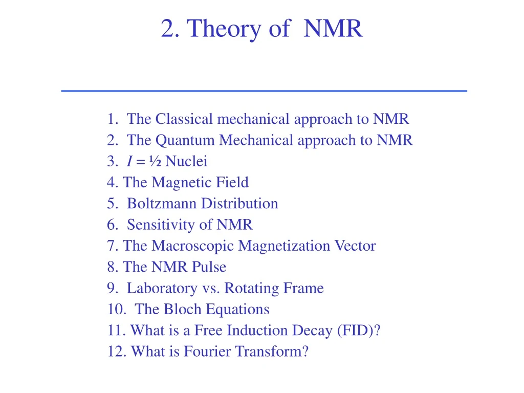
2. Theory of NMR 1. The Classical mechanical approach to NMR 2. The Quantum Mechanical approach to NMR 3. I = ½ Nuclei 4. The Magnetic Field 5. Boltzmann Distribution 6. Sensitivity of NMR 7. The Macroscopic Magnetization Vector 8. The NMR Pulse 9. Laboratory vs. Rotating Frame 10. The Bloch Equations 11. What is a Free Induction Decay (FID)? 12. What is Fourier Transform?
Nuclear Magnetic Resonance Nuclei absorb & emit energy at their resonance frequencies. This method observes the nucleus. A magnetic field is essential for the phenomenon to be observed. 2. Theory of NMR (Dayrit)
A Bird’s Eye View The nucleus and its magnetic moment Through bond coupling B A C Through space coupling 2. Theory of NMR (Dayrit)
Introduction The test substance is placed in a glass tube in the center of a homogeneous magnetic field. A coil is wrapped around the tube. A radio-frequency field (electromagnetic radiation) is imposed on the coil which excites the nuclei of the sample. RF energy can be absorbed or emitted at specific frequencies. This is detected and outputted as the NMR spectrum. The basic NMR set-up Magnetic pole Magnetic pole Sample Electromagnetic excitation and detection 2. Theory of NMR (Dayrit)
What is the physical basis for the NMR signal? Nuclei without a magnetic field: Random orientationof nuclear spins Nuclei in the presence of a magnetic field: Alignment of nuclear spinsalong or against the direction of magnetic field. Magnetic pole Magnetic pole 2. Theory of NMR (Dayrit)
There are two main approaches to NMR theory: • Classical Mechanics: • based on mass and charge of nucleus • represents the nucleus as a bar magnet • useful as a pictorial model but has limited theoretical utility • Quantum Mechanics: • starts with quantized description of a nuclear spin, I • provides a better basis for understanding the NMR phenomenon • necessary to understand the more complex NMR pulse sequences, in particular 2-D NMR 2. Theory of NMR (Dayrit)
1. Classical Mechanical approach to NMR Classical picture. In the presence of an external magnetic field, B0 (z-axis), the nucleus precesses at an angle, , around B0. Such a precessing object possesses an angular momentum, P. If the object has a charge, this gives produces a magnetic moment, . The magnetogyric ratio, , is a constant which is characteristic of the nucleus which arises from the ratio of the magnetic moment, , and the angular momentum, P: =/ P 2. Theory of NMR (Dayrit)
1. Classical Mechanical approach to NMR Limitations of the Classical mechanics approach: • In principle, Classical mechanics (CM) predicts that all nuclei should be observable by NMR. This is not so. • In CM, the only property that distinguishes the various nuclei is their nuclear mass. Classical mechanics predicts that the Larmor frequencies should be inversely proportional to the nuclear mass. This is not so. • CM does not provide a theoretical basis for the phenomena of spin-spin coupling and quadrupolar nuclei. • CM cannot predict transition energies. • CM cannot be used to design NMR pulse experiments. 2. Theory of NMR (Dayrit)
2. Quantum Mechanical approach to NMR • Each atomic nucleus has a nuclear magnetic moment , m, which arises from the spin of the protons and neutrons in the nucleus. The nuclear magnetic moment varies from isotope to isotope of an element. • According to the shell model, protons and neutrons form pairs of opposite total angular momentum. Thus, the magnetic moment of a nucleus with even numbers of both protons and neutrons is zero, while that of a nucleus with an odd number of protons and even number of neutrons (or vice versa) depends on the unpaired proton (or neutron). However, the nuclear magnetic moment is only partly predicted by simple versions of the shell model.. 2. Theory of NMR (Dayrit)
2. Quantum Mechanical approach to NMR • Each nucleus has a spin quantum number, I, which is determined by its nucleus (number of protons and neutrons). Table. Spin quantum numbers, I, of selected nuclei. 2. Theory of NMR (Dayrit)
2. Quantum Mechanical approach to NMR I = ½ Spin ½ nuclei have two quantum states that can be visualized as having the spin axis pointing “up” or “down”. In the absence of an external magnetic field, these two states have the same energy. In the presence of an external magnetic field, B0, and at thermal equilibrium a little less than half of a large population of nuclei will be in the higher state (b) and a little more than one half will be in the lower state (a). (Jacobsen, 2007) 2. Theory of NMR (Dayrit)
Periodic Table of Isotopes: Spin Quantum Numbers, I 2. Theory of NMR (Dayrit)
2. Quantum Mechanical approach to NMR • The nuclear spin quantum number, I, has (2I + 1) values • The magnetic spin quantum numbers, mI: mI= +I, (I- 1), ...-I • Each mI value represents a specific spin state. • The number of mI values represents the number of spin states available to a particular nucleus. 2. Theory of NMR (Dayrit)
2. Quantum Mechanical approach to NMR Table. I, mI and the number of spin states available to a particular nucleus: • Nuclei with I = 0 have no nuclear magnetic properties; they are not observable by NMR (e.g., 12C, 16O, 32S). 2. Theory of NMR (Dayrit)
The magnetic moment, m, is quantized along (2I + 1) orientations with respect to the static magnetic field: m = I (h/2) (rad/T-sec)·(J-sec/rad) = J/T 2. Quantum Mechanical approach to NMR The quantum mechanical description of NMR tells us that the maximum observable component of the angular momentum is: Angular momentum, Pm = I (h/2) (J-sec/rad) where , the magnetogyric ratio, is the proportionality factor between the magnetic moment and the angular momentum. Note: magnetic moment, m = ·Pm 2. Theory of NMR (Dayrit)
Table. Magnetogyric ratios, , of common nuclei. 1 rad = 2p, or approximately 6.28318 2. Theory of NMR (Dayrit)
3. I = ½ systems For I = ½ systems, there are two energy levels: mI = +½ and -½. • The energy separation between these two levels is given by: E = h 0 where o = B0 / 2. • Therefore: E = (h/2) B0 E = 2B0 and for I=½, m = ½ (h/ 2) • Note that according to Quantum Mechanics: • a magnetic field is needed to observe the NMR phenomenon • E B0 2. Theory of NMR (Dayrit)
3. I = ½ systems Splitting of a I = ½ nucleus in a magnetic field. Energy level diagram for I=½. There are two mI levels: ½. These are separated by an energy of: E = 2B0 = (h/2) B0. (Note that E is directly proportional to and B0.) By convention, the upper energy level is designated -½ or , while the lower energy level is +½ or . Some common I = ½ nuclei: 1H, 13C, 19F, 31P 2. Theory of NMR (Dayrit)
3. I = ½ systems What is the energy difference between the two spin states of 1H at different magnetic fields? E = (h/2) B0 where h = 6.632 x 10⁻³⁴ J-s = 26.7519 x 10⁷ rad/T-s B0 (T) 0 MHz (1H) E (x 10-26 J) 1.4 60 3.98 2.35 100 6.68 9.4 400 26.54 2. Theory of NMR (Dayrit)
3. I = ½ systems What is the energy difference between the transitions of 1H and 13C ? E = (h/2) B0 Let B0 = 9.4 T where h = 6.632 x 10⁻³⁴ J-s (x 107 rad/T-s) E (x 10-26 J) E (J/mol) 1H: 26.7519 25.52 0.16 13C: 6.7283 6.67 0.04 • Note: E of 1H is about 4 times that of 13C. 2. Theory of NMR (Dayrit)
3. I = ½ systems What is the energy difference between the transitions of 1H and 13C ? E = (h/2) B0 n0= 100 MHz n0= 400 MHz 2. Theory of NMR (Dayrit)
4. The Magnetic Field A magnetic field is necessary to be able to observe the NMR phenomenon. • Electromagnetic properties are inherent in matter because of their associated electronic properties and magnetic moments. • A nuclear spin with I = ½ is like a microscopic magnet whose orientation is arbitrary until it is placed in a magnetic field. The magnetic field splits it according to its magnetic energy levels. This is called the Zeeman effect. 2. Theory of NMR (Dayrit)
4. The Magnetic Field Effect of magnetic field on Larmor frequency. Splitting of the magnetic energy levels of 1H as a function of 0 (in MHz) vs. magnetic field strength, B0 (in tesla, T). Chemists generally use the 1H Larmor frequency when describing the magnetic field strength. Relationship between magnetic field, B0 (tesla), and the 1H and 13C Larmor frequencies (MHz). Relationship between magnetic field, B0 (tesla) and the 1H Larmor frequency (MHz). 2. Theory of NMR (Dayrit)
4. The Magnetic Field • The NMR phenomenon (nuclear precession) is observable only in the presence of an external magnetic field, B0. • The natural frequency of the precession of a spin is called the Larmor frequency, 0: 0 = B0/ 2 sec-1 = (rad T-1 s-1) (T) where 0 is Larmor frequency, in Hz* is the magnetogyric ratio, in (107 radians/Tesla-sec) B0 is the magnetic field, in Tesla 0 = 20 * The Larmor frequency, designated 0, has units in Hz: * This is also alternatively given in units of (radians/sec): 0 = B0 2. Theory of NMR (Dayrit)
4. The Magnetic Field Table. Larmor frequencies at B0= 2.35 T and 9.4 T. 2. Theory of NMR (Dayrit)
NMR Periodic Table Spin Quantum Numbers, I, and Larmor Frequencies, n0 (at 2.35 T) 2. Theory of NMR (Dayrit)
4. The Magnetic Field 2. Theory of NMR (Dayrit)
5. Boltzmann Distribution I = ½ • In the absence of an external magnetic field (B0 = 0), the nuclear spin energy levels are degenerate (E = 0). When B0>0, the nuclei are split between the nuclear spin energy levels: and . • Using the Boltzmann equation, the population distribution is given as: N/ N = exp (-E /kBT ) where kB = 1.381 x 10⁻²³ J/K T is the absolute temperature in Kelvin • Since E = (h/2) B0, the Boltzmann equation can be rewritten as: N/ N = exp (-hB0/ 2kBT ) 2. Theory of NMR (Dayrit)
5. Boltzmann Distribution • Let us use the Boltzmann equation to calculate the population distribution for: 1H at 60 MHz (1.41 T), T = 300 K: -E = -(6.626 x 10⁻³⁴ J s / 2) (26.75 x 10⁷ rad / T s) (1.41 T) -E = -2.50 x 10⁻²⁵ J per 1H nucleus • At T = 300 K, the Boltzmann equation gives: N/ N = exp{(-2.50 x 10⁻²⁵ J) / [(1.381 x 10⁻²³ J / K) (300 K)]} N/ N = 0.9999400 For 1 million nuclei, 499,985 will be in N and 500,015 will be in N (diff.= 30 spins). To solve: 1. N/ N = 0.9999400 N = (0.9999400) N 2. N + N = 1 2. Theory of NMR (Dayrit)
5. Boltzmann Distribution • Let us compare the population difference for the following: 1H at 400 MHz (9.4 T), T = 300 and 400K: -E = -(6.626 x 10⁻³⁴ J s / 2) (26.75 x 10⁷ rad / T s) (9.4 T) -E = -1.67 x 10⁻²⁴ J • At T = 300 K, the Boltzmann equation gives: N/ N = exp{(-1.67 x 10⁻²⁴ J) / [(1.381 x 10⁻²³ J / K) (300 K)]} N/ N = 0.999600 For 1 million nuclei, 499,900 will be in N and 500,100 will be in N (diff. = 200 spins). • At T = 400 K, the Boltzmann equation gives: N/ N = 0.999698 For 1 million nuclei, 499,924 will be in N and 500,076 will be in N (diff. = 152 spins). 2. Theory of NMR (Dayrit)
5. Boltzmann Distribution • Now, let us use the Boltzmann equation to calculate the populations for: 13C at 9.4 T, T = 300 K: -E = -(6.626 x 10⁻³⁴ J s / 2) (6.72 x 10⁷ rad / T s) (9.4 T) -E = -4.19 x 10⁻²⁵ J per 13C nucleus • At T = 300 K, the Boltzmann equation gives: N/ N = exp{(-4.19 x 10⁻²⁵ J) / [(1.381 x 10⁻²³ J / K) (300 K)]} N/ N = 0.9999899 For 1 million nuclei, 499,975 will be in N and 500,025 will be in N (diff.= 50 spins). 2. Theory of NMR (Dayrit)
5. Boltzmann Distribution • To summarize, the Boltzmann equation predicts the following very important rules regarding the sensitivity of the NMR method: • Magnetogyric ratio, g: NMR is more sensitive towards high g nuclei. • Magnetic field, B0: Higher B0 results in higher sensitivity. • Temperature, K: Higher T leads to lower sensitivity. 2. Theory of NMR (Dayrit)
6. Sensitivity of NMR • The sensitivity of a spectroscopic technique depends on the strength of the absorption signal. The strength of the absorption signal, in turn, depends on the population distribution in the energy levels. • The larger the energy difference between the ground and excited states, the larger is the difference in population. This population difference determines the sensitivity. • Because UV-visible spectroscopy involves electronic energy levels which have relatively large energy separations, it is the most sensitive among the spectroscopic techniques. Sensitivity: UV-visible > Infrared > NMR 2. Theory of NMR (Dayrit)
6. Sensitivity of NMR Table. Comparison of measurement limts for UV-visible, infrared and NMR. TechniqueAmount of sample needed Sensitivity UV-visible ~mg/mL ppm Infrared ~1 mg 0.01% NMR ~1-10 mg/mL % 2. Theory of NMR (Dayrit)
6. Sensitivity of NMR Table. Relative sensitivity of some common I = ½ nuclei. 2. Theory of NMR (Dayrit)
6. Sensitivity of NMR • In sum, there are five factors which affect NMR sensitivity: • the spin quantum number, I; • the magnetogyric ratio of the nucleus, ; • the isotopic abundance, A%; • the strength of the magnetic field, Bo; • the temperature, K. Theoretical parameters Experimental parameters NMR sensitivity [(I+1) / (I2)] (5/2) (A%) (Bo3/2) (K-1) 2. Theory of NMR (Dayrit)
6. Sensitivity of NMR Larmor frequencies of various nuclei at 9.4 T and their relative intensities (where 13C = 1). 13C 2. Theory of NMR (Dayrit)
Periodic Table of Isotopes and their NMR Parameters 2. Theory of NMR (Dayrit)
7. The Macroscopic Magnetization Vector The Boltzmann equation states that the population of spins will be distributed between the quantized lower and upper states. To represent the behavior of large populations, it is more convenient to use a macroscopic magnetization vector, M. While each nucleus has quantized behavior, the entire population of spins exhibits classical (continuous) behavior. M1= 2/3 M2 2. Theory of NMR (Dayrit)
7. The Macroscopic Magnetization Vector From nuclear spin vectors to macroscopic magnetization vectors: the convention: 1. B0 is set along thez-axis. 2. Net spin population is represented by length of the macroscopic magnetization vector, M. 3. Continuous orientation of M. 4. Equilibrium position (ground state) is +z direction; vector is written as M0. +z M +y +x (from: Lambert & Mazzola, 2003) 2. Theory of NMR (Dayrit)
7. The Macroscopic Magnetization Vector 5. Phase of M vector is described by two angles from z-axis and x-axis. 6. Na and Nb are the populations of the lower and upper spin states, respectively. 7. This is not an energy diagram. This is used to represent the orientation of the net macroscopic magnetization vector during the course of the NMR experiment. +z M Nb +y +x Na 2. Theory of NMR (Dayrit)
7. The Macroscopic Magnetization Vector m2 = +½ In a large collection of nuclei (I=½) at equilibrium, each nuclear vector will be rotating (precessing) around the z-axis at the same frequency, 0, but will be doing so randomly. Therefore, they will simply trace a uniform cone around the z-axis, which is represented by M0. +z M Nb +y +x Na m2 = -½ 2. Theory of NMR (Dayrit)
7. The Macroscopic Magnetization Vector m2 = +½ • The macroscopic magnetization vector, M, is the net vector representing all the spins. • M can take any angle although the individual spins can have only quantized orientations of ½. • The z-axis is called the longitudinal axis and the (x,y)- plane is called the transverse plane. • The net (x,y) component of M gives the phase coherence of the spins. M Nb Na m2 = -½ 2. Theory of NMR (Dayrit)
8. The NMR pulse Spectroscopic methods are based on the absorption or emission of a specific frequency of electromagnetic energy by the sample. In the case of NMR, the energy is in the radio frequency (RF) range and the absorbing species are the nuclei. • Pulse FT-NMR utilizes short bursts of RF energy, designated as B1, in the form of pulses to excite a broad range of frequencies. B1 can be considered as a second field. 2. Theory of NMR (Dayrit)
8. The NMR pulse • At equilibrium, M is aligned along B0 (the z-axis), and its projections along the y-x plane, My and Mx = 0. • By convention, the RF pulse, B1, is implemented along the +x-axis. NMR pulse B1 Increase in number of spins in higher spin energy level 2. Theory of NMR (Dayrit)
8. The NMR pulse • A pulse at a right angle to B0 acts as a twisting force on M which causes M to tip away from its equilibrium position into the y'-axis. • A /2 (90o) pulse angle tips M into the x-y plane. The pulse causes a fraction of the spins to precess in-phase. This produces phase coherence. Phase coherence 90 NMR pulse B1 2. Theory of NMR (Dayrit)
8. The NMR pulse • According to the Heisenberg Uncertainty Principle: E .t h where t is the pulse width (PW or p) usually ~ 10-6 s h is Planck’s constant = 6.626 x 10⁻³⁴ J-s • Expanding, we get: (h.) t h (1 /t) • refers to the range of the frequencies which is affected by the pulse, t. A short pulse excites a wide range. A long continuous pulse which excites a narrow range is the same as CW NMR irradiation. 2. Theory of NMR (Dayrit)
8. The NMR pulse In a pulsed NMR experiment, the nuclei are irradiated with an intense B1 field for the duration of the pulse. This causes M to precess at an angle, q, away from B0. During this time, the primary field present is B1, and the precession frequency becomes: w = g B1. 2. Theory of NMR (Dayrit)
8. The NMR pulse The angle or rotation, q, depends on the duration the B1 field is applied, tp. Since w = g B1, it follows that: q = g B1tp 2. Theory of NMR (Dayrit)