Download
1 / 26
260 likes | 319 Views
CHAPTER 2: CHARACTERIZATION OF SEDIMENT AND GRAIN SIZE DISTRIBUTIONS. Sediment diameter is denoted as D; the parameter has dimension [L].

E N D
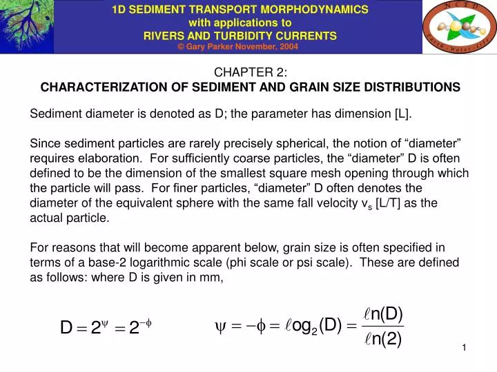
CHAPTER 2: CHARACTERIZATION OF SEDIMENT AND GRAIN SIZE DISTRIBUTIONS Sediment diameter is denoted as D; the parameter has dimension [L]. Since sediment particles are rarely precisely spherical, the notion of “diameter” requires elaboration. For sufficiently coarse particles, the “diameter” D is often defined to be the dimension of the smallest square mesh opening through which the particle will pass. For finer particles, “diameter” D often denotes the diameter of the equivalent sphere with the same fall velocity vs [L/T] as the actual particle. For reasons that will become apparent below, grain size is often specified in terms of a base-2 logarithmic scale (phi scale or psi scale). These are defined as follows: where D is given in mm,
SEDIMENT SIZE RANGES Mineral clays such as smectite, montmorillonite and bentonite are cohesive, i.e. characterized by electrochemical forces that cause particles to stick together. Even silt-sized particles that are do not consist of mineral clay often display some cohesivity due to the formation of a biofilm.
SEDIMENT GRAIN SIZE DISTRIBUTIONS The grain size distribution is characterized in terms of N+1 sizes Db,i such that ff,i denotes the mass fraction in the sample that is finer than size Db,i. In the example below N = 7. Note the use of a logarithmic scale for grain size.
SEDIMENT GRAIN SIZE DISTRIBUTIONS contd. In the grain size distribution of the last slide, the finest size (0.03125 mm) was such that 2 percent, not 0 percent was finer. If the finest size does not correspond to 0 percent content, or the coarsest size to 100 percent content, it is often useful to use linear extrapolation on the psi scale to determine the missing values. Note that the addition of the extra point has increased N from 7 to 8 (there are N+1 points).
SEDIMENT GRAIN SIZE DISTRIBUTIONS contd. The grain size distribution after extrapolation is shown below.
CHARACTERISTIC SIZES BASED ON PERCENT FINER Dx is size such that x percent of the sample is finer than Dx Examples: D50 = median size D90 ~ roughness height To find Dx (e.g. D50) find i such that Then interpolate for x and back-calculate Dx in mm
STATISTICAL CHARACTERISTICS OF SIZE DISTRIBUTION N+1 bounds defines N grain size ranges. The ith grain size range is defined by (Db,i, Db,i+1) and (ff,i, ff,i+1) i (Di) = characteristic size of ith grain size range fi = fraction of sample in ith grain size range
STATISTICAL CHARACTERISTICS OF SIZE DISTRIBUTION contd. = mean grain size on psi scale = standard deviation on psi scale Dg= geometric mean size g = geometric standard deviation ( 1) Sediment is well sorted if g < 1.6 Dg = 0.273 mm, g = 2.17
GRAIN SIZE DISTRIBUTION CALCULATOR A key feature of this e-book is the library of Excel spreadsheet workbooks that go with it. These workbooks allow for implementation of the formulations given in the PowerPoint lectures. Some of these workbooks allow for calculations to be performed directly on the worksheets of the workbook. Others use one or more worksheets as GUI’s (Graphical User Interfaces), where the click of a button executes a code in VBA (Visual Basic for Applications) that is imbedded in the workbook. The first such workbook of this e-book is RTe-bookGSDCalculator.xls. It computes the statistics of a grain size distribution input by the user, including Dg, g, and Dx where x is a specified number between 0 and 100 (e.g. the median size D50 for x = 50). It uses code in VBA (macros) to perform the calculations. You will not be able to use macros if the security level in Excel is set to “High”. To set the security level to a value that allows you to use macros, first open Excel. Then click “Tools”, “Macro”, “Security…” and then in “Security Level” check “Medium”. This will allow you to use macros.
GRAIN SIZE DISTRIBUTION CALCULATOR contd. When you open the workbook RTe-bookGSDCalculator.xls, click “Enable Macros”. The GUI is contained in the worksheet “Calculator”. Now to access the code, from any worksheet in the workbook click “Tools”, “Macro”, “Visual Basic Editor”. In the “Project” window to the left you will see the line “VBA Project (FDe-bookGSDCalculator.xls)”. Underneath this you will see “Module1”. Double-click on “Module1” to see the code in the “Code” window to the right. These actions allow you to see the code, but not necessarily to understand it. In order to understand this course, you need to learn how to program in VBA. Please work through the tutorial contained in the workbook RTe-bookIntroVBA.xls. It is not very difficult! All the input are specified in the worksheet “Calculator”. First input the number of pairs npp of grain sizes and percents finer (npp = N+1 in the notation of the previous slides) and click the appropriate button to set up a table for inputting each pair (grain size in mm, percent finer) in order of ascending size. Once this data is input, click the appropriate button to compute Dg and g. To calculate any size Dx where x denotes the percent finer, input x into the indicated box and click the appropriate button. To calculate Dx for a different value of x, just put in the new value and click the button again.
GRAIN SIZE DISTRIBUTION CALCULATOR contd. This is what the GUI in worksheet “Calculator” looks like.
GRAIN SIZE DISTRIBUTION CALCULATOR contd. If the finest size in the grain size distribution you input does not correspond to 0 percent finer, or if the coarsest size does not correspond to 100 percent finer, the code will extrapolate for these missing sizes and modify the grain size distribution accordingly. The units of the code are “Sub”s (subroutines). An example is given below. Sub fraction(xpf, xp) 'computes fractions from % finer Dim jj As Integer For jj = 1 To np xp(jj) = (xpf(jj) - xpf(jj + 1)) / 100 Next jj End Sub In this Sub, xpf denotes a dummy array containing the percents finer, and xp denotes a dummy array containing the fractions in each grain size range. The Sub computes the fractions from the percents finer. Suppose in another Sub you know the percents finer Ff(i), I = 1..npp and wish to compute the fraction in each grain size range F(i), i = 1..np (where np = npp – 1). The calculation is performed by the statement fraction Ff, f
WHY CHARACTERIZE GRAIN SIZE DISTRIBUTIONS IN TERMS OF A LOGARITHMIC GRAIN SIZE? Consider a sediment sample that is half sand, half gravel (here loosely interpreted as material coarser than 2 mm), ranging uniformly from 0.0625 mm to 64 mm. Plotted with a logarithmic grain size scale, the sample is correctly seen to be half sand, half gravel. Plotted using a linear grain size scale, all the information about the sand half of the sample is squeezed into a tiny zone on the left-hand side of the diagram. Logarithmic scale for grain size Linear scale for grain size
UNIMODAL AND BIMODAL GRAIN SIZE DISTRIBUTIONS The fractions fi(i) represent a discretized version of the continuous function f(), f denoting the mass fraction of a sample that is finer than size . The probability density pf of size is thus given as p = df/d. The example to the left corresponds to a Gaussian (normal) distribution with = -1 (Dg = 0.5 mm) and = 0.8 (g = 1.74): The grain size distribution is called unimodel because the function p() has a single mode, or peak. The following approximations are valid for a Gaussian distribution:
UNIMODAL AND BIMODAL GRAIN SIZE DISTRIBUTIONS contd. A sand-bed river has a characteristic size of bed surface sediment (D50 or Dg) that is in the sand range. A gravel-bed riverhas a characteristic bed size that is in the range of gravel or coarser material. The grain size distributions of most sand-bed streams are unimodal, and can often be approximated with a Gaussian function. Many gravel-bed river, however, show bimodalgrain size distributions, as shown to the upper right. Such streams show a sand mode and a gravel mode, often with a paucity of sediment in the pea-gravel size (2 ~ 8 mm). Plateau Gravel mode Sand mode A bimodal (multimodal) distribution can be recognized in a plot of f versus in terms of a plateau (multiple plateaus) where f does not increase strongly with .
UNIMODAL AND BIMODAL GRAIN SIZE DISTRIBUTIONS contd. The grain size distributions to the left are all from 177 samples from various river reaches in Alberta, Canada (Shaw and Kellerhals, 1982). The samples from sand-bed reaches are all unimodal. The great majority of the samples from gravel-bed reaches show varying degrees of bimodality. Note: geographers often reverse the direction of the grain size scale, as seen to the left. Figure adapted from Shaw and Kellerhals (1982)
GRAVEL-SAND TRANSITIONS As rivers flow from mountain reaches to plains reaches, sediment tends to deposit out, creating an upward concave long profile of the bed and a pattern of downstream fining of bed sediment. Both these patterns are evident in the plots to the right for the Kinu River, Japan (Yatsu, 1955). It is common (but by no means universal) for fluvial sediments to be bimodal, with sand and gravel modes and a relative paucity in the range of pea gravel. In such cases a relatively sharp transition from a gravel-bed stream to a sand-bed stream is often found, often with a concomitant break in slope (Sambrook Smith and Ferguson, 1995, Parker and Cui, 1998). Both these features are evident for the Kinu River. Long profiles of bed elevation, bed slope and median grain size for the Kinu River, Japan. Adapted from Yatsu (1955)
VERTICAL SORTING OF SEDIMENT Gravel-bed rivers such as the River Wharfe often display a coarse surface armor or pavement. Sand-bed streams with dunes such as the one modeled experimentally below often place their coarsest sediment in a layer corresponding to the base of the dunes. River Wharfe, U.K. Image courtesy D. Powell. Sediment sorting in a laboratory flume. Image courtesy A. Blom.
SEDIMENT DENSITY Definitions: = density of water s = material density of sediment s = s/ = specific gravity of sediment R = (s/) – 1 = submerged specific gravity of sediment The defaultsediment density is that of quartz, i.e. 2.65 grams/cm3. This corresponds to the values s = 2.65 and R = 1.65. Two other common natural rock types are basalt (s ~ 2.7 ~ 2.9) and limestone (s ~ 2.6 ~ 2.8). Volcanic sediment often have vugs (large pores), which reduce their effective specific gravity to lower values (e.g. 2.0; in the case of pumice the value can be less than 1.) Rocks containing heavy minerals such as magnetite can have specific gravities of 3 ~ 5. It is common to use lightweight model sediments in the laboratory. Examples include crushed walnut shells (s ~ 1.4), crushed coal (s ~ 1.3 ~ 1.5) and plastic particles (s ~ 1 ~ 2).
SEDIMENT FALL VELOCITY IN STILL WATER Assume a spherical particle with diameter D and fall velocity vs. The downstream impelling force of gravity Fg is: means cD is a function of Revp: see any good fluid mechanics text The resistive drag force is where is the kinematic viscosity of the water and cD is specified by the empirical drag curve for spheres. Condition for equilibrium: where
SEDIMENT FALL VELOCITY IN STILL WATER contd. Untangle the relation: where and where Again this means a functional relationship Reduce to Rf = Rf(Rep) Relation of Dietrich (1982): The original relation also includes a correction for shape.
SOME SAMPLE CALCULATIONS OF SEDIMENT FALL VELOCITY (Dietrich Relation) • g = 9.81 m s-2 • R = 1.65 (quartz) • = 1.00x10⁻⁶ m2 s-1 (water at 20 deg Celsius) = 1000 kg m-3 (water) The calculations to the left were performed withRTe-bookFallVel.xls. Have a look at it. This Excel workbook implements the Dietrich (1982) fall velocity relation. It does not use macros to perform the calculation. In a later chapter of this e-book, this workbook is used to compute fall velocities in the implementation of calculations of suspended sediment concentration profiles.
USE OF THE WORKBOOK FDe-bookFallVel.xls A view of the interface in RTe-bookFallVel.xls is given below. Since VBA is not used, it is not necessary to click a button to perform the calculations. Just fill in the input cells, and the answer will appear in the output cell.
MODES OF TRANSPORT OF SEDIMENT Bed material load is that part of the sediment load that exchanges with the bed (and thus contributes to morphodynamics). Wash load is transported through without exchange with the bed. In rivers, material finer than 0.0625 mm (silt and clay) is often approximated as wash load. Bed material load is further subdivided into bedload and suspended load. Bedload: sliding, rolling or saltating in ballistic trajectory just above bed. role of turbulence is indirect. Suspended load: feels direct dispersive effect of eddies. may be wafted high into the water column.
REFERENCES FOR CHAPTER 2 Dietrich, E. W., 1982, Settling velocity of natural particles, Water Resources Research, 18 (6), 1626-1982. Parker. G., and Y. Cui, 1998, The arrested gravel front: stable gravel-sand transitions in rivers. Part 1: Simplified analytical solution, Journal of Hydraulic Research, 36(1): 75-100. Sambrook Smith, G. H. and R. Ferguson, 1995, The gravel-sand transition along river channels, Journal of Sedimentary Research, A65(2): 423-430. Shaw, J. and R. Kellerhals, 1982, The Composition of Recent Alluvial Gravels in Alberta River Beds, Bulletin 41, Alberta Research Council, Edmonton, Alberta, Canada. Yatsu, E., 1955, On the longitudinal profile of the graded river, Transactions, American Geophysical Union, 36: 655-663.