Week 1a
Week 1a. Affine Term Structure Models. You’ve seen CIR and Vasicek. We’re now going to consider two-factor affine models Basic idea: There are underlying “factors” The interest rate is an affine function of the factors

Week 1a
E N D
Presentation Transcript
Week 1a Affine Term Structure Models
You’ve seen CIR and Vasicek • We’re now going to consider two-factor affine models • Basic idea: There are underlying “factors” • The interest rate is an affine function of the factors • It turns out that there are “essentially” 3 different two-factor affine models
1) Vasicek-like two factor model • We begin with two Brownian motions, and specify two “factor” processes by: • Assume that the B’s are Brownian motion under an equivalent martingale measure. • The B’s satisfy • Finally, the s’s must be strictly positive
We assume the matrix has positive eigenvalues l1,l2 • Finally, we assume the interest rate R is an affine function of the factors: • R(t)=e0+e1X1(t)+e2X2(t)
We’ve got too many “levers” • Fact: different specifications may lead to exactly the same model • Example: just exchange the first two rows • We want to find the a parsimonious representation
Fact: • One parsimonious representation: • This has 6 parameters; the first one had 8. • We restrict l1 and l2 to be positive • We’ll keep the parameters constant
How do we get this reduction? • Look at the text, pp369-373. • For now, we’ll just assume that our model is given in this form.
Bond prices for default-risk-free pure discount bonds • Recall • Because the underlying processes are Markov, all you need to know to compute distributions in the future is today’s state (and the laws of motion). Hence, in principle we can compute B(t,T). • So we can find f for which B(t,T)=f(t,Y1(t),Y2(t)).
Moreover • The discount factor • satisfies dD(t)=-R(t)D(t)dt. • On the previous slide we had • Notice that D(t)B(t,T)=
The right-hand side is clearly a martingale. • Hence: If we compute dt(D(t)B(t,T)), the “dt” term must be 0. • Computing that (and setting the coefficient of “dt” equal to 0) leads to a partial differential equation (10.2.18). This then leads to a system of 3 ordinary differential equations. These equations can be solved.
The solution • f(t,y1,y2)=exp{-y1C1(t)-y2C2(t)-A(t)} • where, if l1 and l2 are not equal, • C1(t)= • C2(t)= • A(t)=