Download
1 / 39
390 likes | 549 Views
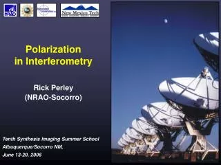
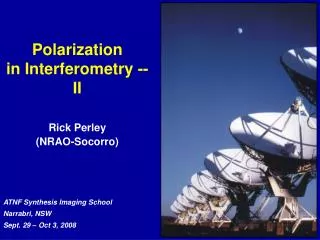
Polarization in Interferometry -- II. Rick Perley (NRAO-Socorro). Introduction. In the last lecture, Dave has: Shown the motivation for doing polarimetry Defined the fundamental definitions that are used in polarimetry. Shown some examples to help illustrate these concepts.

E N D
Polarization in Interferometry -- II Rick Perley (NRAO-Socorro)
Introduction • In the last lecture, Dave has: • Shown the motivation for doing polarimetry • Defined the fundamental definitions that are used in polarimetry. • Shown some examples to help illustrate these concepts. • In this lecture, I will show we actually determine the Stokes parameters with an interferometric array. • To start, we must first define the ‘Stokes Visibilities’, and then review antenna polarization properties.
Stokes Visibilities • Recall the first lecture, where we defined the Visibility, V(u,v), and showed its relation to the sky emission: V(u,v)I (l,m)(a Fourier Transform Pair) • In analogy with this result, let us define the Stokes Visibilities I, Q, U, and V, to be the Fourier Transforms of the true I, Q, U, and V. • Then, the relations between these are: • I I, Q Q, U U, V V • Stokes Visibilities are functions of (u,v), while the Stokes Images are functions of (l,m).
Antenna Polarization • Fundamentally, antennas are polarized. • Their response is sensitive to the polarization of the EM wave • To do polarimetry, the antenna must have two outputs which respond differently to the incoming elliptically polarized wave. • It would be most convenient if these two outputs are proportional to either: • The two linear orthogonal Cartesian components, (EX, EY) or • The two circular orthogonal components, (ER, EL). • For simplicity (for now), let us assume that our antenna’s outputs are indeed perfectly linear, or perfect circular.
Two Orthogonal Outputs per Antenna • To do polarimetry, we must have two outputs from each antenna which respond differently to the polarization state of the incoming EM wave: • In Interferometry, we have two antennas, each with two differently polarized outputs. • We can then form four complex correlations. • What is the relation between these four correlations and the four Stokes’ parameters? Our Generic Sensor Polarizer RCP or XLP LCP or YLP
Four Complex Correlations per Pair of Antennas Antenna 1 Antenna 2 • Two antennas, each with two differently polarized outputs, produce four complex correlations. • From these four outputs, we want to generate four Stokes Visibilities. • How? (feeds) (polarizer) R1 L1 R2 L2 (signal transmission) X X X X (correlators) RR1R2 RR1L2 RL1R2 RL1L2
Orthogonal, Perfectly Linear • Assuming the antenna orientation is fixed to the sky frame, and ignoring calibration: • From these, we can trivially invert and recover the desired Stokes Visibilities. • Note that RXX and RYY have large amplitudes, while RXY and RYX will be small.
Orthogonal, Perfectly Linear • These are: • Note that: • Stokes ‘Q’ – normally a small number, is the difference of two large values, RXX and RYY. • Obtaining an accurate value for Q requires very good gain stability and calibration of the parallel-feed correlations.
Perfectly Circular • So let us continue with our idealizations, and ask what the response is for perfectly circular feeds. • Again assuming the antenna orientation is fixed to the sky, • And again a trivial inversion provides our desired quantities. • Note again that the parallel hand correlations will normally be much larger than the opposite-hand correlations.
Perfectly Circular Feeds • Giving, • Note that now, • It is Stokes ‘V’ which is the difference between two large numbers. • Accurate values for V require high stability and calibration. • The linear polarization visibilities, Q and U, are now the differences between small values – which allows relaxation of the calibration accuracy requirements.
Which System is Best? • The VLA (and EVLA) use circular polarization. • Most new arrays do not (e.g. ALMA, ATCA). • Why? • Antenna feeds are natively linearly polarized. To convert to circular, a quadrature hybrid is needed. This adds cost, complexity, and degrades performance. • For some high frequency systems, or for very wide bandwidth systems, wide-band quarter-wave phase shifters may not be available, or their performance may be too poor. • Linear feeds can give perfectly good linear polarization performance, provided the amplifier/signal path gains are carefully monitored. • Because the parallel-hand correlations with circular feeds do not respond to linear polarization, calibration using linearly-polarized sources is much simplified.
Antenna-Sky Rotation, and the Parallactic Angle • The prior expressions presumed that the antenna feeds are fixed in orientation on the sky. • This is the situation with equatorially mounted antennas. • For antennas with alt-az mounts, the feeds rotate on the sky as they track a source. • The angle between a line of constant azimuth, and one of constant right ascension is called the Parallactic Angle, h : where A is the antenna azimuth, f is the antenna latitude, and d is the source declination. • As the antenna tracks the sky, the azimuth changes, hence so does the parallactic angle.
Including Parallactic Angle (Linear) • Presuming all antennas view the source with the same parallactic angle (not true for VLBI!), the responses from pure polarized antennas are, for linear feeds: • It is easy to solve these for I, Q, U, and V • All four correlations are needed to determine Q and U, but only two are needed for I and V.
Including Parallactic Angle (Circular) • For pure circularly polarized antennas, the expressions are simpler: • Again, solution for the Stokes Visibilities is straightforward. • Only two of the correlations are actually needed for each of the Stokes visibilities.
Real Antennas • The analysis so far has assumed that the antennas are perfectly polarized – their two outputs provide a perfect decomposition of the incoming wave into its orthogonal linear, or orthogonal circular, components. • Sadly, this situation cannot be realized in practice, as antennas are in general cross-polarized. • To incorporate these effects, define the antenna’s polarization parameters: Y and c, where: Y is the polarization position angle, and c is the ellipticity for the particular polarized output of the antenna.
In a more Natural Reference Frame • A more natural description is in a frame (x,h), rotated so the x-axis lies along the major axis of the ellipse. • The three parameters of the ellipse are then: • Ah : the major axis length • Y: the position angle of this major axis, and • tan c = Ax/Ah: the axial ratio • It can be shown that: • The ellipticity c is signed: c > 0 => LEP (clockwise) c < 0 => REP (anti-clockwise)
Antenna Polarization Ellipse • We can thus describe the characteristics of the polarized outputs of an antenna in terms of its antenna polarization ellipses: cR and YR, for the RCP output cL and YL, for the LCP output if the antenna is equipped with nominally circularly polarized feeds, • Or, cx and Yx, for the ‘X’ output, cY and YY, for the ‘Y’ output if the antenna is equipped with nominally linearly polarized feeds.
General Antenna Polarization • The antenna’s polarization is specified by the far-field polarization ellipse resulting from a signal input into each feed. • Note that this will in general be a function of direction!!! q p p q Polarizer q p Reciprocity: An antenna transmits the same polarization that it receives.
Parabolic Antenna Beam Polarization • The beam polarization is due to the antenna/feed geometry. • Grasp8 calculation by Walter Brisken. (EVLA Memo # 58, 2003). • Contour intervals: • V/I = 4%, • Q/I, U/I = 0.2%. • Can be removed – at considerable cost – in imaging. I V/I Q/I U/I
Beam Polarization Profiles Observation of 3C287 offset to half power, at 1485MHz • As 3C287 rotates about the beam: • I (= R+L) is stable to ~1% • V (= R-L) sinusoidally varies with ~8% amplitude • EVLA feed at Az = 0 • VLA feed at Az = 45 • Q, U vary with ~1.5% amplitude.
Generalized Interferometer Response • We are now in a position to show the most general expression for the output of a complex correlator for an interferometer comprising arbitrarily polarized antennas to partially-polarized astronomical signals. • This is a complex expression (in all senses of that adjective), and I will make no attempt to derive, or even justify it. • The expression is completely general, valid for a linear system.
Here it is! The terms shown are 4 of the 16 elements of the matrix (often erroneously termed the Mueller Matrix) relating the four complex correlations to the four Stokes Visibilities. This relation was derived by Morris, Radhakrishnan and Seielstad (1964). Rpqis the complex output from the interferometer, for polarizations p and q from antennas 1 and 2, respectively. Y and c are the antenna polarization major axis and ellipticity for states p and q. I,Q, U, and V are the Stokes Visibilities Gpq is a complex gain, including the effects of transmission and electronics
Reduction for Simple Cases • In general each of the four complex correlations responds to all four Stokes visibilities. • For perfectly polarized antennas, these expressions quickly reduce to the examples already shown. • For example, for perfectly linear feeds, c = 0, YV = 0, YH = p/2. • While for perfectly circular feeds, cR = -p/4, cL = p/4 • I leave to you students the effort of actually showing this, and in the extension for including the parallactic angle.
An Alternate Representation • A cleaner and more intuitive representation of the general response is found if we adopt a circular basis, and make the substitutions: • The b terms represent the deviation of the antenna polarization from perfect circularity. • the f represent the orientation of the antenna polarization ellipse in the antenna’s frame. • The term YP is the parallactic angle. • The C and S terms form the elements of the Jones Matrix. Then define:
The Matrix Formulation • After some (considerable) labor, we find: • Where:
What Good is all This??? • It allows easy derivation for any general case. • Simplification One: Assume all parallactic angles equal. • Simplification Two: Assume perfect circular systems: • Simplification Three: Assume perfect linear systems: b = 0 b = p/4 fR = 0 fL = p/2
Case 3: Nearly circular system • If our engineers have made nearly perfect circular polarizers, then: • All ‘C’ terms are ~ 1 • All ‘S’ terms are very small: |S| << 1 • If we then ignore all 2nd order products in S (S1S2* = 0), and ignore all products between S and Q, S and U, and S and V: then: This leads to a well-known (and often used) approximation:
‘Nearly’ Circular Feeds (small D approximation) • We get: • Our problem is now clear. The desired cross-hand responses are contaminated by a term proportional to ‘I’. • Stokes ‘I’ is typically 20 to 100 times the magnitude of ‘Q’ or ‘U’. • We must either make the S terms much smaller than this, or be able to correct for them to an accuracy better than this. • To do accurate polarimetry, we must determine these S-terms, and remove their contribution.
Some Comments • Determination of the S (leakage, or cross-polarization) terms is normally done either by: • Observing a source of known (I,Q,U) intensity, or • Multiple observations of a source of unknown (I,Q,U), and allowing the rotation of parallactic angle to separate the two terms. • The latter method works well, as: • In the frame of the antenna, the cross-polarization term is constant over time, while • The source linear polarization term has a phase which rotates at twice the parallactic angle. • Note that for each, the absolute value of S cannot be determined – they must be referenced to an arbitrary value.
Nearly Perfectly Linear Feeds • We can follow the same exercise for nearly perfect linears, but the physical interpretation is not the same. • In this case, assume that the ellipticity is very small (c << 1), and that the two feeds (‘dipoles’) are nearly perfectly orthogonal. • We then define a *different* set of S-terms: • The angles jY and jXare the angular offsets from the exact horizontal and vertical orientations, w.r.t. the antenna.
This gives us … • I’ll spare you the full equation set, and show only the results after the same approximations used for the circular case are employed.
Some Comments on Linears • The problem is the same as for the circular case: • The parallel-hand correlations are not affected by the cross-polarization (to first order), while • the derivation of the Q, U, and V Stokes’ visibilities is contaminated by a leakage of the much larger I visibility into the cross-hand response. • Calibration is similar to the circular case: • If Q, U, and V are known, then the equations can be solved directly for the Ds. • If the polarization is unknown, then the antenna rotation can again be used (over time) to separate the polarized response from the leakage response.
Comments on Cross-Polarization • Determination and removal of these ‘leakage’ terms is a well established and successful procedure. • The origins of the cross-polarization lie in the electronics (primarily in the cryogenic components), and in the antenna structures themselves. • These components are very stable in temperature and over time, so we expect the ‘S’ terms to be stable – as they nearly always are. • If the first-order approximations are used to solve for the S terms, then they must be referenced to one antenna. Only the (complex) differences can be observed – which is all that are needed. • Determining *absolute* S terms is possible – easily if the parallactic angles are very different (VLBI) – with more difficulty if they are similar.
How Well Does This Work? 3C147, a strong unpolarized source … I Q Peak = 4 mJy, s = 0.8 mJy Peak at 0.02% level – but not noise limited! Peak = 21241 mJy, s = 0.21 mJy Max background object = 24 mJy
A Typical Baseline X-Pol Response Before Polarization Calibration After Polarization Calibration 2.1% and stable 0.3% stable residual! Amplitude 125 degrees and stable 250 degree rotation! Phase
3C287 at 1465 MHZ I and V with the VLA I V 5% False V! 9% Peak = 6982 mJy, s = 0.21 mJy Max Bckg. Obj. = 87 mJy Peak = 6 mJy, s = 0.16 mJy Background sources falsely polarized.
Removal of Polarization Beams • Sanjay Bhatnagar has implemented an algorithm to permit removal of pointing variations and beam polarization • In Stokes I, primary problem is variation in pointing. • Simulated results: After Before
Stokes V correction • In Stokes ‘V’, primary problem is the beam squint. • Bhatnagar algorithm effectively removes the false polarization. • The same software will correct Q, and U images. Before Correction After Correction
A Summary • Polarimetry is a little complicated. • But, the polarized state of the radiation gives valuable information into the physics of the emission. • Well designed systems are stable, and have low cross-polarization. • Such systems easily allow estimation of polarization to an accuracy of 1 part in 10000. • Beam-induced polarization can be corrected in software – development is under way. • We can surely do better with a little more effort…