Parallel Algorithms and Computing Selected topics
Parallel Algorithms and Computing Selected topics. Parallel Architecture. References. An introduction to parallel algorithms Joseph Jaja Introduction to parallel computing Vipin Kumar, Ananth Grama, Anshul Gupta, George KArypis Parallel sorting algorithms Selim G. Akl. Models.


Parallel Algorithms and Computing Selected topics
E N D
Presentation Transcript
Parallel Algorithms and ComputingSelected topics Parallel Architecture
References An introduction to parallel algorithms Joseph Jaja Introduction to parallel computing Vipin Kumar, Ananth Grama, Anshul Gupta, George KArypis Parallel sorting algorithms Selim G. Akl
Models Three models: Graphs (DAG : Directed Acyclic Graph) Parallel Randon Access Machine Network
Graphs Not studied here
Parallel Architecture Parallel random access machine
Parallel Randon Access Machine • Flynn classifies parallel machines based on: • Data flow • Instruction flow • Each flow can be: • Single • Multiple
Parallel Randon Access Machine • Flynn classification Data flow Instruction flow
Mémoire Globale (Shared – Memory) P1 P2 Pp Parallel Randon Access Machine • Extend the traditional RAM (Random Access Memory) machine • Interconnection network between global memory and processors • Multiple processors
Parallel Randon Access Machine Characteristics • Processors Pi (i (0 i p-1 ) • each with a local memory • i is a unique identity for processor Pi • A global shared memory • it can be accessed by all processors
Parallel Randon Access Machine Types of operations: • Synchronous • Processors work in locked step Fat each step, a processor is active or idle Fsuited for SIMD and MIMD architectures • Asynchronous • processors have local clocks • needs to synchronize the processors F suited for MIMD architecture
Parallel Randon Access Machine • Example of synchronous operation Algorithm : Processor i (i=0 … 3) Input : A, B i processor id Output : (1) C Begin If ( B==0) C = A Else C = A/B End
Parallel Randon Access Machine Initial Processeur 0 Processeur 1 Processeur 2 Processeur 3 A : 5 B : 0 C : 0 A : 4 B : 2 C : 0 A : 2 B : 1 C : 0 A : 7 B : 0 C : 0 Step 1 Processeur 0 Processeur 1 Processeur 2 Processeur 3 A : 5 B : 0 C : 5 (Actif, (B=0) A : 4 B : 2 C : 0 (Inactif, (B0) A : 2 B : 1 C : 0 (Inactif, (B0) A : 7 B : 0 C : 7 (Actif, B=0) (active B =0) (idle B 0) (idle B 0) (active B = 0)
Step 2 Processeur 0 Processeur 1 Processeur 2 Processeur 3 A : 5 B : 0 C : 5 A : 4 B : 2 C : 2 A : 2 B : 1 C : 2 A : 7 B : 0 C : 7 Parallel Randon Access Machine (idle B =0) (active B 0) (active B 0) (idle B = 0)
Parallel Randon Access Machine Read / Write conflicts • EREW : Exclusive - Read, Exclusive -Write • no concurrent ( read or write) operation on a variable • CREW : Concurrent – Read, Exclusive – Write • concurrent reads allowed on same variable • exclusive write only
Parallel Randon Access Machine • ERCW : Exclusive Read – Concurrent Write • CRCW : Concurrent – Read, Concurrent – Write
Parallel Randon Access Machine Concurrent write on a variable X • Common CRCW : only if all processors write the same value on X • SUM CRCW : write the sum all variables on X • Random CRCW : choose one processor at random and write its value on X • Priority CRCW : processor with hign priority writes on X
Parallel Randon Access Machine Example: Concurrent write on X by processors P1 (50 X) , P2 (60 X), P3 (70 X) • Common CRCW ou ERCW : Failure • SUM CRCW : X is the sum (180) of the written values • Random CRCW : final value of X { 50, 60, 70 }
Parallel Randon Access Machine Basic Input/Output operations • On global memory • global read (X, x) • global write (Y, y) • On local memory • read (X, x) • write (Y, y)
Example 1: Matrix-Vector product • Matrix-Vector produt Y = AX • A is a nXn matrix • X = [ x1, x2, …, xn] a vector of n elements • p processeurs ( pn ) and r = n/p • Each processor is assigned a bloc of r= n/p elements
P1 P2 Pp Example 1: Matrix-Vector product Global memory A1,1 A1,2 … A1,n A2,1 A2,2 … A2,n …….. A n,1 An,2 ... An,n X1 X2 …. Xn Y1 Y2 …. Yn X = Processors
A1,1 A1,2 … A1,n ……. Ar,1 A2,2 … A2,n ……. A(p-1)r,1 A(p-1),2 … A(p-1),n …….. A pr,1 Apr,2 ….Apr,n r lignes A1 Ap A1 A2 …. Ap = A = r lignes Example 1: Matrix-Vector product Partition A in p blocks Ai • Compute p partial products in parallel • Processor Pi compute the partial product Yi = Ai * X
A1,1 A1,2 … A1,n ……. Ar,1 A2,2 … A2,n Y1 Y2 …. Yr X1 X2 …. Xn X1 X2 …. Xn X1 X2 …. Xn X X X P1 Yr+1 Yr+2 …. Y2r P2 Ar+1,1 Ar+1,2 … Ar+1,n ……. A2r,1 A2r,2 … A2r,n Y(p-1)r+1 Y(p-1)r+2 …. Ypr Pp A(p-1)r,1 A(p-1)r,2 …A(p-1)r,n ……. Apr,1 Apr,2 … Apr,n Example 1: Matrix-Vector product Processeur Pi computes Yi = Ai * X
Example 1: Matrix-Vector product Solution requires : • p concurrents reads of vector X • each processor Pi makes an exclusive read of block Ai = A [((i-1)r +1) : ir, 1:n] • Each processor Pi makes an exclusive write on block Yi = Y[((i-1)r +1) : ir ] Required architecture : PRAM CREW
Example 1: Matrix-Vector product Algorithm: processor Pi (i=1,2, …, n) • Input • A : nxn matruix in global memory • X : a vector in global memory • Output • y = AX (y is a vector in global memory) • Local variables • i : Pi processor id • p: number of processors • n : dimension of A and X • Begin • 1. Global read ( x, z) • 2. global read (A((i-1)r + 1 : ir, 1:n), B) • 3. calculer W = Bz • 4. global write (w, y(i-1)r+1 : ir)) • End
Example 1: Matrix-Vector product Analysis • Computation cost Ligne 3: O( n2/p) opérations arithmétiques by Pi r lignes X n opérations ( avec r = n/p) • Communication cost Ligne 1 : O(n) numbers transferred from global to local memory by Pi Ligne 2 : O(n2/p) numbers transferred from global to local memory by Pi Ligne 4 : O(n/p) numbers transferred from global to local memory by Pi • Overall: Algorithm run in O(n2/p) time
Example 1: Matrix-Vector product Other way to partition the matrix is vertically • Ai and X are split into blocks • A1, A2, … Ap • X1, X2 … Xp • Solution in two phases : • Compute partial products Z1 =A1X1, … Zp = ApXp • Synchronize the processors • Add partial results to get Y Y= AX = Z1 + Z2 + … + Zp
r columns r columns …….. Example 1: Matrix-Vector product A1,1 … A1,r A2,1 … A2,r An,1 … An,r X1 … Xr * Y1 Y2 …. Yn Processor P1 A1,(p-1)r +1 ... A1,pr A2,(p-1)r +1 ... A2,pr An,(p-1)r +1 ... An,pr X(p-1)r +1 ... Xpr * Synchronization Processor Pp
Example 1: Matrix-Vector product Algorithm: processor Pi (i=1,2, …, n) • Input • A : nxn matruix in global memory • X : a vector in global memory • Output • y = AX (* y: vector in global memory *) • Local variables • i : Pi processor id • p: number of processors • n : dimension of A and X • Begin • 1. Global read ( x( (i-1)r +1 : ir) , z) • 2. global read (A(1:n, (i-1)r + 1 : ir), B) • 3. compute W = Bz • 4. Synchronize processors Pi (i=1, 2, …, n) • 5. global write (w, y(i-1)r+1 : ir)) • End
Example 1: Matrix-Vector product Analysis • Work out the details • Overall: Algorithm run in O(n2/p) time
Example 2: Sum on the PRAM model An aray A of n = 2k numbers A PRAM machine with n processor Compute S = A(1) + A(2) + …. + A(n) Construct a binary tree to compute the sum in log2n time
S=B(1) P1 P1 B(1) B(1) B(1) B(4) B(3) B(2) B(1) =A(1) B(2) =A(2) B(1) =A(1) B(2) =A(2) Example 2: Sum on the PRAM model Level >1, Pi compute B(i) = B(2i-1) + B(2i) Level 1, Pi B(i) = A(i) B(2) P2 P1 P1 P3 P4 P2 B(1) =A(1) B(2) =A(2) B(1) =A(1) B(2) =A(2) P1 P2 P3 P4 P5 P6 P7 P8
Example 2: Sum on the PRAM model Algorithm processor Pi ( i=0,1, …n-1) • Input • A : array of n = 2k elements in mémoire global • Output • S : où S= A(1) + A(2) + …. . A(n) • Local variables Pi • n : • i : processor Pi identity • Begin • 1. global read ( A(i), a) • 2. global write (a, B(i)) • 3. for h = 1 to log n do • if ( i ≤ n / 2h ) then begin • global read (B(2i-1), x) • global read (b(2i), y) • z = x +y • global write (z,B(i)) • end • 4. if i = 1 then global write(z,S) • End
Parallel Architecture Network model
Network model Characteristics • Communication structure is important • Network can be seen as a graph G=(N,E): • Node i N is a processor • Edge (i,j)E represents a two way communication between processors i and j • Basi communication operation • Send (X, Pi) • Receive(X, Pi) No global shared memory
… P2 P1 P3 Pn Network model n processors Linear array … P2 P1 P3 Pn n processor ring
Network model n2 processors Grid … P12 P11 P13 P1n … P22 P21 P23 P2n … P32 P31 P33 P3n … Pn2 Pn1 Pn3 Pnn n2 processors Torus: columns and rows are n rings
Network model n=2k hypercube (P7) (P6) (P2) (P3) (P4) (P5) (P1) (P0)
Network model n2 processors Grid … P12 P11 P13 P1n … P22 P21 P23 P2n … P32 P31 P33 P3n … Pn2 Pn1 Pn3 Pnn n2 processors Torus: columns and rows are n rings
Exemple 1: Matrix-Vector Product on linear array • A=[aij] an nxn matrix, i,j [1,n] • X=[xi] i [1,n] • Compute
a44 a43 a42 a41 a34 a33 a32 a31 a24 a23 a22 a21 a14 a13 a12 a11 . . . . . . x4 x3 x2 x1 P2 P1 P3 P4 Exemple 1: Matrix-Vector Product on linear array Systolic array algorithm for n=4
Exemple 1: Matrix-Vector Product on linear array • At step j, xj enters the processor P1. At step j, processor Pi receives • (when possible) a value from its left and a value from the top. • It updates its partial as follows: • Yi = Yi + aij*xj , j=1,2,3, …. • Values xj and aij reach processor i at the same time at step (i+j-1) • (x1, a11) reach P1 at step 1 = (1+1-1) • (x3, a13) reach P1 at setep 3 = (1+3-1) • In general, Yi is computed at step N+i-1
Exemple 1: Matrix-Vector Product on linear array • The computation is completed when x4 and a44 reach processor P4 at • Step N + N –1 = 2N-1 • Conclusion: The algorithm requires (2N-1) steps. At each step, active processor • Perform an addition and a multiplication • Complexity of the algorithm: O(N)
Step x1 1 x1 x2 2 x2 x1 x3 3 x3 x2 x1 4 x4 4 4 4 4 y1 = a1j*xj y4 = a4j*xj y2 = a2j*xj y3 = a3j*xj x4 x3 x2 x1 5 J=1 J=1 J=1 J=1 x4 x3 x1 x2 6 x1 x2 x4 x3 7 P2 P2 P2 P2 P2 P2 P2 P1 P1 P1 P1 P1 P1 P1 P3 P3 P3 P3 P3 P3 P3 P4 P4 P4 P4 P4 P4 P4 Exemple 1: Matrix-Vector Product on linear array
P2 P2 P2 P2 P2 P2 P2 P1 P1 P1 P1 P1 P1 P1 P3 P3 P3 P3 P3 P3 P3 P4 P4 P4 P4 P4 P4 P4 Exemple 1: Matrix-Vector Product on linear array Systolic array algorithm: Time-Cost analysis 1 Add; 1 Mult; active: P1 idle: P2, P3, P4 2 Add; 2 Mult; active: P1, P2 idle: P3, P4 3 Add; 3 Mult; active: P1, P2,P3 idle: P4 4 Add; 4 Mult; active: P1, P2,P3 P4 idle: 3 Add; 3 Mult; active: P2,P3,P4 idle: P1 2 Add; 2 Mult; active: P3,P4 idle: P1,P2 1 Add; 1 Mult; active: P4 idle: P1,P2,P3
Step x1 1 x1 x2 2 x2 x1 x3 3 x3 x2 x1 4 x4 x4 x3 x2 5 x4 x3 6 x4 7 P2 P2 P2 P2 P2 P2 P2 P1 P1 P1 P1 P1 P1 P1 P3 P3 P3 P3 P3 P3 P3 P4 P4 P4 P4 P4 P4 P4 Exemple 1: Matrix-Vector Product on linear array Systolic array algorithm: Time-Cost analysis 1 Add; 1 Mult; active: P1 idle: P2, P3, P4 2 Add; 2 Mult; active: P1, P2 idle: P3, P4 3 Add; 3 Mult; active: P1, P2,P3 idle: P4 4 Add; 4 Mult; active: P1, P2,P3 P4 idle: 3 Add; 3 Mult; active: P2,P3,P4 idle: P1 2 Add; 2 Mult; active: P3,P4 idle: P1,P2 1 Add; 1 Mult; active: P4 idle: P1,P2,P3
Exemple 2: Matrix multiplication on a 2-D nxn Mesh • Given two nxn matrices A = [aij] and B = [bij], i,j [1,n], • Compute the product C=AB , where C is given by :
Exemple 2: Matrix multiplication on a 2-D nxn Mesh • At step i, Row i of A (starting with ai1) is entered from the top into column i (into processor P1i) • At step j, Column j of B (starting with b1j) is entered from the left into row j (to processor Pj1) • The values aik and bkj reach processor (Pji) at • step (i+j+k-2). • At the end of this step, aik is sent down and bkj is sent right.
a44 a43 a42 a41 . . . a34 a33 a32 a31 . . a24 a23 a22 a21 a14 a13 a12 a11 . b41 b3 b21 b11 (1,4) (1,2) (1,3) (1,1) . b42 b32 b22 b12 (2,1) (2,2) (2,3) (2,4) . . b43 b33 b23 b13 (3,1) (3,2) (3,3) (3,4) . . b44 b34 b24 b14 (4,1) (4,2) (4,3) (4,4) Exemple 2: Matrix multiplication on a 2-D nxn Mesh Example: Systolic mesh algorithm for n=4 STEP 1
a44 A a34 a43 a24 a33 a42 b41 b31 b21 b11 a14 a41 a23 a32 b12 b32 b22 b42 a13 a31 b43 a22 b33 b23 b13 • a12 b44 b34 a21 b14 b24 B • a11 Exemple 2: Matrix multiplication on a 2-D nxn Mesh Example: Systolic mesh algorithm for n=4 STEP 5
Exemple 2: Matrix-Vector multiplication on a ring Analysis • To determine the number of steps for completing the multiplication of the matrice, we must find the step at which the terms ann and bnn reach rocessor Pnn. • Values aik and bkj reach processor Pji at i+j+k-2 • Substituing n for i,j,k yields : n + n + n – 2 = 3n - 2 • Complexity of the solution: O(N)