Developing Predictive Hurricane Models: Fine-Tuning with Recursive Least Squares Method
This study aims to minimize numerical errors in hurricane models to better quantify the impact of model parameters on predicted fields. Employing observational data, such as lightning strikes, combined with various data assimilation approaches, the research addresses the dominant temporal errors arising from time-splitting techniques. A physics-based preconditioner enhances Krylov solver efficiency for modeling idealized hurricanes, leading to faster-than-real-time simulations. Key approximations and advanced microphysical modeling techniques are discussed, focusing on resolving cloud-edge dynamics and improving overall model accuracy.

Developing Predictive Hurricane Models: Fine-Tuning with Recursive Least Squares Method
E N D
Presentation Transcript
Towards Developing a “Predictive” Hurricane Model or the “Fine-Tuning” of Model Parameters via a Recursive Least Squares Procedure • Goal: Minimize numerical errors within a model to be able to accurately quantify the impacts of model parameters on the predicted fields • Methodology: Use observational data, i.e., lighting, in combination with various data assimilation approaches to determine model parameters
Temporal Errors • Are typically the dominant errors • Produced by time-splitting • Grow rapidly in-time for time-steps above the fastest time-scale; determined by the smallest grid spacing in the model, i.e., vertical sound wave propagation
Time-Splitting All terms, advection, diffusion, and various sources must be at the same time-level; otherwise time-splitting is the result…
How to Avoid Time-Splitting Errors • First, use a time-stepping procedure that does not produce these errors, i.e., Runge-Kutta • Second, time-scales must be resolved with regard to the accuracy of the temporal integrator • Third, use Newton’s method to determine if time scales are being resolved!
Newton’ Method Current models typically produce an order one Newton error, i.e., f(x)=x-sin(x)=1
Physics-Based Preconditioner • For problems with a large separation in time scales, convergence of a Krylov solver can be extremely slow • A physics-based preconditioner is designed to remove fast time scales in an efficient manner • For a single phase Navier-Stokes equation set, the preconditioner was designed to remove sound waves only • With a physics-based preconditioner active,theJFNK procedure is somewhat like a “predictor-corrector” type algorithm • Entire numerical approach has been used in the simulation of idealized hurricanes employing Navier-Stokes
Cloud field from an idealized smooth hurricane simulation Reisner et al., 2005, MWR, 133, 1003-1022
An Example of a Physics-Based Preconditioner Used Within the Hurricane Model Faster than Real-time 20 times speed up Reisner et al., 2005, MWR, 133, 1003-1022
5.0 s time step 2.5 s time step Large Errors in Potential Temperature, As large as errors in physical models? 1.0 s time step 60.0 s time step
Key Approximations in Idealized Hurricane Model • Microphysical model involved a simple conversion between water vapor and total cloud substance • Mesh Reynolds number in both horizontal and vertical directions where near 0.1 to resolve smoothly resolve cloud edges
A More “Complex” Smooth Bulk Microphysical Model • Reworked the Reisner/Thompson et al. microphysical model so that it is smooth or “numerically differentiable” implying… • An individual parameterization cannot take out more cloud substance, i.e., rain, than exists in a given cell • Sum of all parameterizations cannot take out more than exists in a given cell • Fastest time scale of an individual parameterization is the sound wave time-scale • Cloud quantities do not go to zero outside the cloud, i.e., f(x)=x-sin(x)
A multi-phase particle-based approach is being used to model spectra In hurricanes
Cloud-edge Problem • Time-scales can be very fast near cloud boundaries, i.e., boundary is not resolved • Eulerian advection is the problem, including positive definite schemes and flux-corrected transport (FCT) schemes • Diffusion is the answer…increases time & spatial scales • But, unlike the previous example, high levels of diffusion need not be added everywhere
Advection canIntroduce a Small DynamicalTime Scale Near Cloud Edges • Advection (ADV) is typically of opposite sign to diffusion (DIFF) near cloud edges • By monitoring this time scale, accuracy and efficiency of a given numerical procedure is maximized • Can be tied to the convergence of Newton’s method • Most cloud models use time steps that exceed this time scale, FCT enables this…
Edge Problem (Con’t)FCT Versus Cloud-Edge Diffusion • FCT procedure implicitly adds diffusion near cloud edges, but is not time accurate • Cloud-edge diffusion explicitly adds diffusion near edges,but may add too much diffusion… • But, by knowing how much diffusion is being added, evaporation can be limited • Which approach is better? Depends on whether one cares about resolving time and spatial scales during a simulation and also how implicit diffusion influences a given feature
Evaporation combined with fast condensational growth can lead to sharp cloud edges Quadratic interpolation leads to oscillations near the edges, must either resolve the edges via diffusion or use linear interpolation to minimize oscillations… the basis for flux-corrected advective transport (FCT) Most cloud models employ FCT to keep cloud variables positive and free from oscillations!
Cloud Edge Diffusionfrom Dimensional Analysis Diffusion operator in x direction for cloud water field… Adds a resolved spatial scale! • Two approaches for determining closure coefficient: • Constant, • Advective procedure
Cloud-edge diffusion associated with the movement of a 1-D cloud
Observations from DYCOMS-II, from Steven et al. (2005, MWR, 133, 1443-1462) Almost all cloud models produce too high of a cloud base
3-D Isosurface of Cloud Water from Smooth Cloud Model 3-D Isosurface of Cloud Water from Traditional Cloud Model
Time averaged X-Z Cross-Sections of Cloud Water from the Smooth Cloud Model Using Various Time Step Sizes Time averaged X-Z Cross-Sections of Cloud Water from the Traditional Cloud Model Using Various Time Step Sizes
Smooth Approach: Little Differences in Cloud Features with Different Time Step Sizes
Traditional Approach: Big Differences in Cloud Features with Different Time Step Sizes
Error in Cloud Water from Smooth Cloud Model Error in Cloud Water from Traditional Cloud Model
Idealized Hurricane Simulations-Next Iteration • Base equation set-Navier-Stokes+new smooth cloud model • Constant resolution in horizontal (10 km) and vertical (300 m) • Predictive fields were initialized using sounding data representative of the atmosphere during the rapid intensification phase of Rita • “Bogus-vortex” was used to help spin-up hurricanes
Key Tuning Parameter • Vertical heat and moisture transport are key to rapid intensification • Coarse model resolution implies that these processes must be parameterized • Hence, the key tuning parameter in the model is related to how quickly these quantities are “diffused” in the vertical direction…helps force formation of hot towers • Parameter must be reasonably smooth…
U Isosurfaces & Wind Vector Field
W Isosurfaces & Wind Vector Field
Rain Isosurfaces & Wind Vector Field
Rita Simulations Questions? • For a “real” case, does rapid intensification still occur? • Does the model develop bands? • How sensitive is the model to variations in the model parameter…?
Rita Setup • Bogus vortex, Key West Nexrad radar data (processed by Steve Guimond) for eyewall, LASA data for bands • DBZ radar data was used to initialize rain water and graupel via simple functional relationships • LASA data was used to initialize water vapor, I.e., where lighting was present within a column water vapor was added to force saturation
Rita Setup (Con’t) • 4 km horizontal resolution & 300 m vertical resolution • All fields were initialized from the same sounding data used to initialize the idealized simulations • Currently investigating impact of diffusion parameter as well as band initialization on intensification
Rain Isosurfaces & Wind Vector Field
W Isosurfaces & Wind Vector Field
W Isosurfaces & Wind Vector Field
Conclusions & Future Work • Intensification of a modeled hurricane at coarse resolution is extremely sensitive to vertical diffusion • Time errors can be important during rapid intensification • Is rapid intensification predictable? Maybe, with reasonable observational data and advanced data assimilation approaches