Download
1 / 39
400 likes | 649 Views
Scene recognition by inexact graph matching. Celso C. Ribeiro * Claudia Boeres Isabelle Bloch. IV ALIO/EURO Workshop on Applied Combinatorial Optimization Pucón, Chile, November 4-6, 2002. Summary. Motivation and applications Optimal graph matching formulation

E N D
Scene recognition by inexact graph matching Celso C. Ribeiro * Claudia Boeres Isabelle Bloch IV ALIO/EURO Workshop on Applied Combinatorial Optimization Pucón, Chile, November 4-6, 2002 Scene recognition by inexact graph matching
Summary • Motivation and applications • Optimal graph matching formulation • Model: objective function and constraints • Randomized construction algorithm • Local search • GRASP heuristic • Numerical results • Current and future work Scene recognition by inexact graph matching
Motivation and applications • Recognition and understanding of complex scenes require a detailed description of … • … the objects involved • … the spatial relationships between the objects • The diversity of the forms of the same object in different instantiations of a scene, and also the similarities of different objects in the same scene, make the relationships between objects of prime importance to help the recognition of objects with similar appearance. Scene recognition by inexact graph matching
Motivation and applications • Graph-based representations often used for scene representation: • Nodes represent the objects in the scene. • Edges represent the relationships between the objects. • Relevant information is extracted from the scene and represented by relational attributed graphs. • Model-based recognition: both the model and the scene are represented by graphs. Graph matching problem Scene recognition by inexact graph matching
Motivation and applications • Matching: graph or subgraph isomorphism • The assumption of a bijection between the elements in two instantiations of the same scene is too strong for some problems. • Usually, the model has a schematic aspect. • Construction of the image graph often relies on segmentation techniques that mail fail in accurately representing the image in meaningful entities, therefore no isomorphism can be expected. • Recognition can be better expressed as an inexact (non-bijective) graph matching problem. Scene recognition by inexact graph matching
Motivation and applications • Application: • Recognition of brain structures from 3D magnetic resonance images previously processed by a segmentation model (ENST and hospital Saint Vincent de Paul, Paris) • Model is an anatomical atlas: nodes represent the anatomical structures, while edges represent the spatial relationships between them. • Inaccuracies: oversegmented image, unexpected objects found (e.g. pathologies), expected objects not found, deformations, imprecise attributes Scene recognition by inexact graph matching
(a) Normal brain (b) Pathological brain (c) Brain atlas Motivation and applications • Axial slices of a brain (each grey level corresponds to a unique connected structure): middle dark structures (lateral ventricles) are much bigger in (b) than in (a), the white hyper-signal structure (tumor) in (b) does not appear in (a) or (c). Scene recognition by inexact graph matching
Motivation and applications • Other applications: • Aerial or satellite image interpretation using a map • Face recognition • Character recognition Scene recognition by inexact graph matching
Optimal graph matching formulation • Attributed graphs: one single vertex for each image region • Typical attributes: adjacencies, distances, relative positions, grey levels • Vertex similarities and edge similarities are computed from the values of the attributed graphs, relating each pair of vertices and each pair of edges (one from the model, the other from the image). Scene recognition by inexact graph matching
Optimal graph matching formulation • Model: G1=(N1,E1) • Oversegmented image: G2=(N2,E2), with |N2|>|N1| • Assign one single node of N1 to each node of N2: • Set of nodes associated with i N1: Scene recognition by inexact graph matching
Optimal graph matching formulation • Edges (a,b) E1 and (p,q) E2 are associated if node a N1 is associated with p N2 and node b N1is associated with q N2. Scene recognition by inexact graph matching
Optimal graph matching formulation • Search for the optimal graph matching which best represents the scene recognition is based on similarity values. Scene recognition by inexact graph matching
Optimal graph matching formulation • Similarity matrices: sv(i,j ): vertex-similarity between vertices i N1 and j N2. se(u,v ): edge-similarity between edges u = (a,b ) E1 and v = (c,d ) E2. • A good matching is a solution in which the vertex associations and the edge associations correspond to high similarity values. Scene recognition by inexact graph matching
node-similarities contribution edge-similarities contribution Model: objective function Scene recognition by inexact graph matching
node-similarities contribution: High similarity associations are privileged: sv(i,j ) high xij = 1 maximizes Low similarity associations are penalized: sv(i,j ) low xij = 0 maximizes Model: objective function Scene recognition by inexact graph matching
Constraint (1): For every j N2, there exists exactly one node i N1 such that xij = 1, i.e. Model: constraints • Each vertex of N2 has to be associated with exactly one vertex of N1: • Image segmentation is performed by an appropriate algorithm which preserves the boundaries. • In consequence, it avoids situations in which one region of the segmented image is located in the frontier of two adjacent regions of the model and no undersegmentation occurs. Scene recognition by inexact graph matching
Model: constraints • Vertices of N2 associated with the same vertex of N1 should be all connected among themselves: • An oversegmentation method can split an object into several pieces, but it does not change their relative positions (connectivity constraint). Constraint (2): For every i N1, the graph induced by A (i ) in G2 = (N2,E2) is connected. Scene recognition by inexact graph matching
Constraint (4): For every i N1, there exists at least one node j N2 such that xij = 1, i.e. Model: constraints • Pairs of vertices with null similarity cannot be associated: Constraint (3): sv(i,j ) = 0 xij = 0. • All objects in the model should appear in the image: Scene recognition by inexact graph matching
Randomized construction algorithm • MaxTrials: maximum number of attempts to build a feasible solution. • Repeat for at most MaxTrials attempts: • Set A (i ) = for every i N1. • Randomly select a node jN2 and set N2N2 – {j }. • Randomly select a node iN1, until sv(i,j ) > 0 and the graph induced in G2 by A (i ) {j } is connected. • Set A (i ) A (i ) {j }. • If N2 ≠ go back to step 2 above. • If A (i ) ≠ i N1 and A -1(j ) ≠ j N2, then stop. Scene recognition by inexact graph matching
Randomized construction algorithm • The algorithm stops and returns the first feasible solution found within at most MaxTrials attempts. • The algorithm enforces feasibility, good solutions are not necessarily obtained. • It may also be extended to return the best among the first MaxSolutions feasible solutions built. • Each attempt has time complexity . Scene recognition by inexact graph matching
Randomized construction algorithm Scene recognition by inexact graph matching
Test problems • 12 test problems • Some randomly generated, others from real problems associated with medical images • Two difficult instances with isolated nodes • Largest instance has |N1|=50 and |E1|=88, |N2|=250 and |E2|=1681. • Construction algorithm is very fast and very often finds a feasible solution in the first attempt. • Instances with isolated nodes are harder, but even in these cases a feasible solution is built. Scene recognition by inexact graph matching
Test problems: I-6 (human brain) Model: 12 vertices 42 edges Image: 95vertices 1434 edges Scene recognition by inexact graph matching
Test problems: I-7 (muscle) Model: 14 vertices 27 edges Image: 28vertices 63 edges Scene recognition by inexact graph matching
Test problems: I-7 (muscle) model oversegmented image Scene recognition by inexact graph matching
Best of 100 first feasible solutions: 12 regions correctly recognized Best of ten first feasible solutions: 5 nodes correctly recognized First feasible solution: 4 regions correctly recognized Test problems: I-7 (feasible solutions) Scene recognition by inexact graph matching
Local search • Solutions built by the construction algorithm are not necessarily optimal. • Local search algorithm successively replaces the current solution by a better one in a neighborhood of the first, terminating at a local optimum. • First improving strategy: the current solution is replaced by the first neighbor whose cost function value improves that of the current solution. Scene recognition by inexact graph matching
Local search: neighborhoods • Neighborhood A: all solutions that can be obtained from the current one by modifying A -1(j )for some node j N2 (the new node associated with j has to enforce all feasibility constraints). • Neighborhood B: all solutions that can be obtained from the current one by exchanging the nodes A -1(p) and A -1(q ) of N1, currently associated with nodes p and q of N2. Scene recognition by inexact graph matching
Local search: neighborhoods Neighborhood A: associate a new node (a) with node 2 Neighborhood B: exchange the nodes b and c associated with nodes 4 and 7 Scene recognition by inexact graph matching
Local search • VND procedure using neighborhoods A and B and a first improving strategy: • Start with a solution built by the construction algorithm. • Move to the first improving solution in neighborhood A of the current solution until a local optimum is found. • If the current solution is also locally optimal with respect to neighborhood B, then stop. • Otherwise, move to the first improving solution in neighborhood B and go back to step 2. Scene recognition by inexact graph matching
Local search • Each local search iteration (neighborhood search and move) has time complexity . • Local search improved the solution value for all test problems. Scene recognition by inexact graph matching
Local search applied to the best of the 100 first feasible solutions built: 13 regions correctly recognized (out of 28) Local search: I-7 Scene recognition by inexact graph matching
GRASP heuristic • GRASP: multistart metaheuristic • Each iteration has two phases: construction and local search • MaxIterations: maximum number of iterations • Repeat for MaxIterations iterations: • Build a feasible solution using the randomized construction algorithm. • Use the local search procedure to improve the solution built. • Update the best solution found. Scene recognition by inexact graph matching
GRASP heuristic • Good solutions obtained with a few hundred GRASP iterations. • Improved solutions for all test problems • Small computation times • Problem I-7, 20000 GRASP iterations: 216 seconds on a Pentium II 450 MHz Scene recognition by inexact graph matching
GRASP heuristic • Solution values for α = 0.9: construction algorithm with MaxTrials = 500, first improving local search strategy, and 200 GRASP iterations Scene recognition by inexact graph matching
GRASP heuristic: I-7 20000 GRASP iterations, with local search starting from the first feasible solution built in the construction phase: 26 regions correctly recognized (out of 28) Scene recognition by inexact graph matching
GRASP heuristic: 1000 iterations Problem I-6 Problem I-7 Scene recognition by inexact graph matching
Current and future current work • Improved construction algorithm incorporating a greedy (randomized) insertion criterion • Improvement of the GRASP heuristic using path-relinking • Parallelization on a 64-node Linux cluster using the MPI library for communication • Comparison with other approaches in the literature, in particular with genetic algorithms • Application to the recognition of facial features Scene recognition by inexact graph matching
Slides and publications • Slides of this talk can be downloaded from: http://www.inf.puc-rio/~celso/talks • Papers about the randomized construction heuristic with local search for scene recognition (shortly) available at: http://www.inf.puc-rio.br/~celso/publicacoes (also available: other papers about GRASP, parallelization, and path-relinking) Scene recognition by inexact graph matching