Download
1 / 12
130 likes | 253 Views
Indexing in Spatial Databases and Query Processing. Query Processing. Efficient algorithms to answer spatial queries Common Strategy - filter and refine Filter Step: Query Region overlaps with MBRs (minimum bounding rectangles) of B,C and D

E N D
Query Processing • Efficient algorithms to answer spatial queries • Common Strategy - filter and refine • Filter Step: Query Region overlaps with MBRs (minimum • bounding rectangles) of B,C and D • Refine Step: Query Region overlaps with B and C • - For reducing computation time: • - It is easier (computationally cheaper) to compute the intersection between • a query region and a rectangle rather than between the query region • and an arbitrary, irregular shaped, spatial object. Fig 1.8
File Organization and Indices • DBMS have been designed to handle very large amounts of data • The fundamental difference in how algorithms are designed in a • GIS data analysis vs a database environment • A difference between GIS and SDBMS assumptions • GIS algorithms: • Main focus is minimizing the computation time • Assuming that entire dataset is residing in main memory • SDBMS: dataset is on secondary storage e.g disk • Main focus is on I/O time • I/O time is the time required to transfer data from a disk to the main • memory • finite main memory infinite disk • SDBMS uses spatial indices to efficiently search large spatial datasets in DB
File Organization and Indices • programmer’s view-point: computation time • DBMS designer’s view-point: I/O time • CPU-bound • I/O bound • Computation time • I/O time
Indexing • Consider secondary storage as a book • The smallest unit of transfer between the disk and main memory is a page. And records of a tble are like structured lines of text on the page • At anytime some pages reside in main meory, some at the disk • To accelerate the search DB uses index • DBMS can fetch all the pages spanned by a table and scan them line by line until the record is found • Or search in the index and for a desired key word and go directly to the page specified in the index. • Index entries in a book are sorted in alphabetical order • Similarly if the index is built on numbers, like the social security number, then they can be numerically numbered.
Spatial Indexing: Search Data-Structures • Choice for spatial indexing: for query optimization • B-tree is a hierarchical collection of ranges of linear keys, e.g. numbers • B-tree index is used for efficient search of traditional data • Crucially depends on the existence of an order in the indexing field. • See the difference between binary tree and B-tree • Each node represents page B-tree R- tree
Spatial Indexing: Search Data-Structures • Which nodes are index pages and which nodes are data pages • If a page holds m keys, then the height ? • O(logm n) • What is n? • WHY B-TREE IS NOT APPROPRIATE FOR INDEXING SPARIAL DATA
Minimum Bounding Rectangle Study Area Minimum Bounding Rectangles
R-tree for Spatial Data Indexing • Because natural order does not exist in multidimensional space, the B-tree can not be used directly to create an index of spatial objects. • R-tree data structure was one of the first index structure specifically designed to handle multidimensional extended objects • R-tree provides better search performance yet! • R-tree is a hierarchical collection of rectangles
R-tree: Example Examples of R – Tree Index of polygons
Query Optimization • Query Optimization • A spatial operation can be processed using different strategies • Computation cost of each strategy depends on many parameters • Example Query: • Find the names of all female senators who own a business • SELECT S.name FROM Senator S, Business B • WHERE S.soc-sec = B.soc-sec AND S.gender = ‘Female’ • Here, there is a selection query and a join query • Optimization • Process (S.gender = ‘Female’) before (S.soc-sec = B.soc-sec ) • Do not use index for processing (S.gender = ‘Female’)
Multi-scan Query Example • Find all senators who serve a district of area greater than 300 • square miles and who own business within the district. • Spatial join example • SELECT S.name FROM Senator S, Business B • WHERE S.district.Area() > 300 AND Within(B.location, S.district) • Here, composition of two sub-queries, a range query and a spatial join • Which one is first?