Download
1 / 25
260 likes | 295 Views
Explore the theoretical treatment and numerical experiments regarding the charged particle beams and galaxy dynamics. The study discusses the validity of the theoretical foundation and presents conclusions drawn from the research conducted in the seminar. Insights on phase mixing of regular and chaotic orbits, as well as foundational theories in chaotic-mixing theory, are elaborated upon. The text delves into the geometric approach and presents a simpler picture of the chaotic-mixing rate. Application examples to beams, χ model galactic potential, and simulations in different potentials are also detailed.

E N D
RAPID EVOLUTION OF • CHARGED-PARTICLE BEAMS AND GALAXIES • Courtlandt L. Bohn, FNAL • (in collaboration with • Henry E. Kandrup, Univ. of Florida, • Rami A. Kishek, Univ. of Maryland) • Introduction • Theoretical Treatment • Numerical Experiments vs. Theory • Validity of Theoretical Foundation • Conclusions • Jefferson Lab Center for Advanced Studies of Accelerators Seminar, 12 October 2001
The introductory remarks begin with a synopsis of the five-beamlet experiment done at the University of Maryland in the early 1990s. These experiments are described in detail in M. Reiser, Theory and Design of Charged Particle Beams (Wiley, NY, 1994), pp. 479-491. One can see from the figures therein that the beamlets dissipate about 1 meter away from the cathode and are completely gone at the end of the 5 meter transport channel. By contrast, a simple calculation shows that the relaxation time scale from two-body interactions corresponds to about 1 kilometer. Thus, the experiments appear to show a rapid migration to some sort of quasiequilibrium with a smooth density in a short time scale that apparently depends little on the degree of rms mismatch of the beam to the transport channel. Similar behavior may also be inferred from images of large self-gravitating stellar systems.
MANIFESTATIONS OF PHASE MIXING • Phase Mixing of Regular Orbits: • Reversible, in principle, • Initially nearby trajectories diverge as ~tp, • Time scale τ ~ (ωmax - ωmin)-1. • Phase Mixing of Chaotic Orbits: • Irreversible, • Initially nearby orbits diverge as ~eχt, • Time scale ~χ-1, the “largest Lyapunov exponent”.
EXAMPLE: CHAOTIC vs. REGULAR ORBITS Ensemble of chaotic orbits Ensemble of regular orbits [H.E. Kandrup, in Galaxy Dynamics, D.R. Merritt, M. Valluri, J.A. Sellwood, Eds. ASP Conference Series, 1999, 182, pp. 197-208.]
FOUNDATION FOR CHAOTIC-MIXING THEORY [Review article: L. Casetti, M. Pettini, E.G.D. Cohen, Phys. Rep.337, 237 (2000).] • Basic Idea: Particle orbits are geodesics in a Riemannian manifold. • Key assumptions and approximations: • The particle orbits (e.g., geodesics) are generically chaotic. • The manifold's effective curvature is locally deformed but otherwise constant. • The effective curvature reflects a gaussian stochastic process. • Long-time-averaged properties of the curvature are calculable as phase-space averages over an invariant measure, taken to be the microcanonical ensemble. This list is tantamount to presuming the system is "globally chaotic".
BASIC IDEA OF GEOMETRIC APPROACH:
CHAOTIC-MIXING RATE: [L. Casetti, R. Livi, and M. Pettini, Phys. Rev. Lett.74, 375 (1995)].
A SIMPLER PICTURE • Use Hamilton’s equations: • Introduce small perturbations: • Result is evolution equations of the form: from which • The crucial assumption is that this can be modeled as a • stochastic-oscillator equation.
MODEL GALACTIC POTENTIAL Homogeneous ellipsoid with massive black hole at its centroid: MBH = black-hole mass; E = particle energy = V(r) at orbital turning points. In simulations choose ε per computational considerations, but: In mixing-time theory choose ε = 0.5(MBH)1/3 ↔ Vellipsoid ~ 0.1VBH at r = ε to preserve "regularity” near the black hole.
MODEL 3D GALACTIC POTENTIAL Theory vs. Simulation numerical E = 1.0 theoretical E = 0.6 E = 0.4 ωx2 = 0.75, ωy2 = 1.0, ωz2 = 1.25 [H.E. Kandrup, I.V. Sideris, and C.L. Bohn, PRE (submitted)]
MODEL 2D GALACTIC POTENTIAL Theory vs. Simulation E = 1.0 E = 0.6 E = 0.4 Orbits are restricted to (x,y)-plane.
TOOL FOR SIMULATING BEAMS • Self-consistent Particle-in-Cell code (WARP). • Place localized “ensembles” of test particles in 4D • phase space. • Track moments of each ensemble and trajectories of • randomly-selected particles from each ensemble. • Obtain numerical convergence (4M particles total, with • 20k particles/ensemble). • Can explore wide variety of conditions: mismatch, • periodic focusing, anisotropy, bends, arbitrary • initial distributions, etc.
THE “CONTROL EXPERIMENT” [R.A. Kishek, et. al., PAC’01] Uniform Focusing: Energy = 10 keV, Current = 100 mA dc, Emittance (90%) = 50 μm, Radius = 1 cm, Space-charge tune = 0.13, λp = 1.14 m, λβo = 1.63 m, λβ = 12.57 m. Blue ensemble comprises interacting particles; other ensembles comprise test particles. Plots at distances of 0.0, 11.52, 51.84, 100.8, 169.9 m (top to bottom).
MIXING IN ISOTROPIC PHASE SPACE Evolution of natural logarithm of the “emittance” moment: [R.A. Kishek, C.L. Bohn, I. Haber, P.G. O'Shea, M. Reiser, H. Kandrup, Proc. 2001 PAC]
Equipartitions in 5 m Damps in 50 m INTRODUCE ANISOTROPY: ex = 2ey • [R.A. Kishek, P.G. O'Shea, and M. Reiser, Phys. Rev. Lett. 85, 4514 (2000).]
MIXING IN ANISOTROPIC PHASE SPACE Evolution of natural logarithm of the “emittance” moment: mixes thoroughly in ~50 m e-folds in ~2 m
PARTICLE ORBITS IN PHASE SPACE Isotropic Case (red ensemble) Anisotropic Case (green ensemble) x-y x-x' x'-y'
HOW INVALID ARE THE ASSUMPTIONS IN LOWER-DIMENSIONAL SYSTEMS? [H.E. Kandrup, I.V. Sideris, and C.L. Bohn, PRE (submitted)] • Example -- Generalized Dihedral Potential: • Curvature and its variance versus particle energy E: Microcanonical Orbital Data D = 2 D = 3
DIHEDRAL POTENTIAL (cont.) • Gaussian Distribution of Curvatures • for D>2: Orbital Data Microcanonical E = 1 E = 6 D = 2 D = 6 D = 4,5,6 Orbital Data Microcanonical
DIHEDRAL POTENTIAL (cont.) • Numerical vs. Theoretical Lyapunov Exponents (E = 1): D = 3 D = 2 D = 4 D = 5 Rescaled autocorrelation time D = 6 D = 6
SOME OBSERVATIONS • Theoretical mixing rates are correct within factors ~2. • Minor modifications do not yield vastly different results. • No single modification will give perfect agreement for • all potentials and energies. • Largest discrepancies relate to large populations of • “sticky” orbits. BUT -- In real systems, external noise • and internal irregularities work to overcome “stickiness”. • Results seem to be principally sensitive to the estimated • autocorrelation time. KEY POINT: The results corroborate the idea that chaotic mixing reflects a parametric instability that can be modeled by a stochastic-oscillator equation.
SUMMARY AND CONCLUSIONS • What have we done? • Uncovered the mechanism of chaotic mixing. • Estimated mixing time scales in time-independent potentials; compared them to simulations. • Found that when chaotic mixing is active, the density profile determines its rapidity. • Found suggestive hints of chaotic mixing in beam simulations. • It seems possible to use beams to infer physics of rapid • "relaxation" in other N-body systems, e.g., galaxies. • We are currently planning experiments on UMER to • further the understanding of chaotic mixing.