Download
1 / 53
530 likes | 546 Views
This lecture introduces the concepts of query evaluation and optimization in database applications, including operator evaluation, query optimizer, projection hashing, and sorting. Topics discussed include catalog management, cost-based query subsystem, query plan generation, and plan cost estimation.

E N D
Carnegie Mellon Univ.Dept. of Computer Science15-415/615 - DB Applications C. Faloutsos – A. Pavlo Lecture#13: Query Evaluation
Today's Class • Catalog (12.1) • Intro to Operator Evaluation (12.2-3) • Typical Query Optimizer (12.6) • Projection: Sorting vs. Hashing (14.3.2) CMU SCS 15-415/615
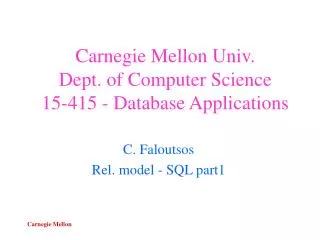
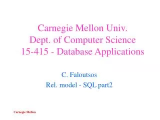
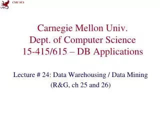
Catalog Manager Cost-based Query Sub-System Select * From Blah B Where B.blah = blah Queries Query Parser Query Optimizer Plan Generator Plan Cost Estimator Schema Statistics Query Plan Evaluator Faloutsos
Catalog Manager Cost-based Query Sub-System Select * From Blah B Where B.blah = blah Queries Query Parser Query Optimizer Plan Generator Plan Cost Estimator Schema Statistics Query Plan Evaluator Faloutsos
Catalog: Schema • What would you store? • Info about tables, attributes, indices, users • How? • In tables!Attribute_Cat (attr_name: string, rel_name: string; type: string; position: integer) CMU SCS 15-415/615
Catalog: Schema • What would you store? • Info about tables, attributes, indices, users • How? • In tables!Attribute_Cat (attr_name: string, rel_name: string; type: string; position: integer) See INFORMATION_SCHEMAdiscussion from Lecture #7 CMU SCS 15-415/615
Catalog: Statistics • Why do we need them? • To estimate cost of query plans • What would you store? • NTuples(R): # records for table R • NPages(R): # pages for R • NKeys(I): # distinct key values for index I • INPages(I): # pages for index I • IHeight(I): # levels for I • ILow(I), IHigh(I): range of values for I CMU SCS 15-415/615
Catalog: Statistics • Why do we need them? • To estimate cost of query plans • What would you store? • NTuples(R): # records for table R • NPages(R): # pages for R • NKeys(I): # distinct key values for index I • INPages(I): # pages for index I • IHeight(I): # levels for I • ILow(I), IHigh(I): range of values for I CMU SCS 15-415/615
Today's Class • Catalog (12.1) • Intro to Operator Evaluation (12.2-3) • Typical Query Optimizer (12.6) • Projection: Sorting vs. Hashing (14.3.2) CMU SCS 15-415/615
Query Plan Example SELECT cname, amt FROM customer, account WHERE customer.acctno = account.acctno AND account.amt > 1000 Relational Algebra: pcname, amt(samt>1000 (customer⋈account)) CMU SCS 15-415/615
Query Plan Example SELECT cname, amt FROM customer, account WHERE customer.acctno = account.acctno AND account.amt > 1000 p cname, amt s amt>1000 ⨝ acctno=acctno CUSTOMER ACCOUNT CMU SCS 15-415/615
Query Plan Example SELECT cname, amt FROM customer, account WHERE customer.acctno = account.acctno AND account.amt > 1000 “On-the-fly” p cname, amt “On-the-fly” s amt>1000 Nested Loop ⨝ acctno=acctno File Scan File Scan CUSTOMER ACCOUNT CMU SCS 15-415/615
Query Plan Example SELECT cname, amt FROM customer, account WHERE customer.acctno = account.acctno AND account.amt > 1000 p Each operator iterates over its input and performs some task. The output of each operator is the input to the next operator. s ⨝ CUSTOMER ACCOUNT CMU SCS 15-415/615
Operator Evaluation • Several algorithms are available for different relational operators. • Each has its own performance trade-offs. • The goal of the query optimizer is to choose the one that has the lowest “cost”. Next Class: How the DBMS finds the best plan. CMU SCS 15-415/615
Operator Execution Strategies • Indexing • Iteration (= seq. scanning) • Partitioning (sorting and hashing) CMU SCS 15-415/615
Access Paths • How the DBMS retrieves tuples from a table for a query plan. • File Scan (aka Sequential Scan) • Index Scan (Tree, Hash, List, …) • Selectivity of an access path: • % of pages we retrieve • e.g., Selectivity of a hash index, on range query: 100% (no reduction!) CMU SCS 15-415/615
Operator Algorithms • Selection: • Projection: • Join: • Group By: • Order By: CMU SCS 15-415/615
Operator Algorithms • Selection: file scan; index scan • Projection: hashing; sorting • Join: • Group By: • Order By: CMU SCS 15-415/615
Operator Algorithms • Selection: file scan; index scan • Projection: hashing; sorting • Join: many ways (loops, sort-merge, etc) • Group By: • Order By: CMU SCS 15-415/615
Operator Algorithms • Selection: file scan; index scan • Projection: hashing; sorting • Join: many ways (loops, sort-merge, etc) • Group By: hashing; sorting • Order By: sorting CMU SCS 15-415/615
Operator Algorithms Next Class • Selection: file scan; index scan • Projection: hashing; sorting • Join: many ways (loops, sort-merge, etc) • Group By: hashing; sorting • Order By: sorting Today Next Class Today Today CMU SCS 15-415/615
Today's Class • Catalog (12.1) • Intro to Operator Evaluation (12.2-3) • Typical Query Optimizer (12.6) • Projection: Sorting vs. Hashing (14.3.2) CMU SCS 15-415/615
Query Optimization • Bring query in internal form (eg., parse tree) • … into “canonical form” (syntactic q-opt) • Generate alternative plans. • Estimate cost for each plan. • Pick the best one. CMU SCS 15-415/615
Query Plan Example SELECT cname, amt FROM customer, account WHERE customer.acctno = account.acctno AND account.amt > 1000 p cname, amt s amt>1000 ⨝ acctno=acctno CUSTOMER ACCOUNT CMU SCS 15-415/615
Query Plan Example SELECT cname, amt FROM customer, account WHERE customer.acctno = account.acctno AND account.amt > 1000 p p cname, amt cname, amt s ⨝ acctno=acctno amt>1000 ⨝ acctno=acctno amt>1000 s CUSTOMER ACCOUNT CUSTOMER ACCOUNT CMU SCS 15-415/615
Today's Class • Catalog (12.1) • Intro to Operator Evaluation (12.2,3) • Typical Query Optimizer (12.6) • Projection: Sorting vs. Hashing (14.3.2) CMU SCS 15-415/615
Duplicate Elimination • What does it do, in English? • How to execute it? SELECT DISTINCT bname FROM account WHEREamt > 1000 pDISTINCTbname(samt>1000 (account)) Not technically correct because RA doesn’t have “DISTINCT” CMU SCS 15-415/615
Duplicate Elimination SELECT DISTINCT bname FROM account WHEREamt > 1000 p DISTINCT bname • Two Choices: • Sorting • Hashing s amt>1000 ACCOUNT CMU SCS 15-415/615
Sorting Projection p DISTINCT bname s amt>1000 X ACCOUNT Filter Sort RemoveColumns Eliminate Dupes CMU SCS 15-415/615
Alternative to Sorting: Hashing! • What if we don’t need the order of the sorted data? • Forming groups in GROUPBY • Removing duplicates in DISTINCT • Hashing does this! • And may be cheaper than sorting! (why?) • But what if table doesn’t fit in memory? CMU SCS 15-415/615
Hashing Projection • Populate an ephemeral hash table as we iterate over a table. • For each record, check whether there is already an entry in the hash table: • DISTINCT: Discard duplicate. • GROUPBY: Perform aggregate computation. • Two phase approach. CMU SCS 15-415/615
Phase 1: Partition • Use a hash function h1 to split tuples into partitions on disk. • We know that all matches live in the same partition. • Partitions are “spilled” to disk via output buffers. • Assume that we have B buffers. CMU SCS 15-415/615
Phase 1: Partition B-1 partitions Redwood p DISTINCT bname Downtown Downtown s amt>1000 h1 ⋮ ACCOUNT Filter RemoveColumns Hash Perry CMU SCS 15-415/615
Phase 2: ReHash • For each partition on disk: • Read it into memory and build an in-memory hash table based on a hash function h2 • Then go through each bucket of this hash table to bring together matching tuples • This assumes that each partition fits in memory. CMU SCS 15-415/615
Phase 2: ReHash Redwood p DISTINCT bname Downtown Downtown s amt>1000 Partitions From Phase 1 h2 h2 h2 ⋮ ACCOUNT Perry Hash Table Eliminate Dupes CMU SCS 15-415/615
Analysis • How big of a table can we hash using this approach? • B-1 “spill partitions” in Phase 1 • Each should be no more than B blocks big CMU SCS 15-415/615
Analysis • How big of a table can we hash using this approach? • B-1 “spill partitions” in Phase 1 • Each should be no more than B blocks big • Answer: B∙(B-1). • A table of N blocks needs about sqrt(N) buffers • What assumption do we make? CMU SCS 15-415/615
Analysis • How big of a table can we hash using this approach? • B-1 “spill partitions” in Phase 1 • Each should be no more than B blocks big • Answer: B∙(B-1). • A table of N blocks needs about sqrt(N) buffers • Assumes hash distributes records evenly! • Use a “fudge factor” f >1 for that: we need • B ~ sqrt( f ∙N) CMU SCS 15-415/615
Analysis • Have a bigger table? Recursive partitioning! • In the ReHash phase, if a partition i is bigger than B, then recurse. • Pretend that i is a table we need to hash, run the Partitioning phase on i, and then the ReHash phase on each of its (sub)partitions CMU SCS 15-415/615
Recursive Partitioning Hash the overflowingbucket again ⋮ Hash h1’ h1 h2 h2 h2 h2 h2 CMU SCS 15-415/615
Real Story • Partition + Rehash • Performance is very slow! • What could have gone wrong? CMU SCS 15-415/615
Real Story • Partition + Rehash • Performance is very slow! • What could have gone wrong? • Hint: some buckets are empty; some others are way over-full. CMU SCS 15-415/615
Hashing vs. Sorting • Which one needs more buffers? CMU SCS 15-415/615
Hashing vs. Sorting • Recall: We can hash a table of size N blocks in sqrt(N) space • How big of a table can we sort in 2 passes? • Get N/B sorted runs after Pass 0 • Can merge all runs in Pass 1 if N/B ≤ B-1 • Thus, we (roughly) require: N ≤ B2 • We can sort a table of size N blocks in about space sqrt(N) • Same as hashing! CMU SCS 15-415/615
Hashing vs. Sorting • Choice of sorting vs. hashing is subtle and depends on optimizations done in each case • Already discussed optimizations for sorting: • Heapsort in Pass 0 for longer runs • Chunk I/O into large blocks to amortize seek+RD costs • Double-buffering to overlap CPU and I/O CMU SCS 15-415/615
Hashing vs. Sorting • Choice of sorting vs. hashing is subtle and depends on optimizations done in each case • Another optimization when using sorting for aggregation: • “Early aggregation” of records in sorted runs • Let’s look at some optimizations for hashing next… CMU SCS 15-415/615
Hashing: We Can Do Better! • Combine the summarization into the hashing process - How? CMU SCS 15-415/615
Hashing: We Can Do Better! • During the ReHash phase, store pairs of the form <GroupKey, RunningVal> • When we want to insert a new tuple into the hash table: • If we find a matching GroupKey, just update the RunningVal appropriately • Else insert a new <GroupKey, RunningVal> CMU SCS 15-415/615
Hashing Aggregation SELECT acctno,SUM(amt) FROM account GROUP BYacctno Running Totals Redwood Downtown Downtown Partitions From Phase 1 h2 h2 h2 ⋮ Perry Hash Table Final Result CMU SCS 15-415/615
Hashing Aggregation • What’s the benefit? • How many entries will we have to handle? • Number of distinct values of GroupKeys columns • Not the number of tuples!! • Also probably “narrower” than the tuples CMU SCS 15-415/615