Download
1 / 45
470 likes | 662 Views
Nash Equilibrium: Illustrations. Cournot’s Model of Oligopoly. Single good produced by n firms Cost to firm i of producing q i units: C i ( q i ), where C i is nonnegative and increasing If firms’ total output is Q then market price is P(Q), where P is nonincreasing

E N D
Cournot’s Model of Oligopoly • Single good produced by n firms • Cost to firm i of producing qi units: Ci(qi), where Ci is nonnegative and increasing • If firms’ total output is Q then market price is P(Q), where P is nonincreasing • Profit of firm i, as a function of all the firms’ outputs:
Cournot’s Model of Oligopoly Strategic game: • players: firms • each firm’s set of actions: set of all possible outputs • each firm’s preferences are represented by its profit
Example: Duopoly • two firms • Inverse demand: • constant unit cost: Ci(qi) = cqi, where c < a
Example: Duopoly Recall for a perfectly competitive firm, P=MC, so a – Q = c, or Q = a – c. Recall for a monopolist, MR=MC, so a – 2Q = c, or Q = (a – c)/2.
Example: Duopoly • Best response function is: Same for firm 2: b2(q) = b1(q) for all q.
Example: Duopoly Nash equilibrium: Pair (q*1, q*2) of outputs such that each firm’s action is a best response to the other firm’s action or q*1 = b1(q*2) and q*2 = b2(q*1) Solution: q1 = ( a - c - q2)/2 and q2 = (a - c - q1)/2 q*1 = q*2 = (a - c)/3
Example: Duopoly Conclusion: • Game has unique Nash equilibrium: (q*1, q*2) = (( a - c)/3, (a - c)/3) • At equilibrium, each firm’s profit is p = ((a - c)2)/9 • Total output 2/3(a- c) lies between monopoly output (a - c)/2 and competitive output a - c.
Cournot’s Model of Oligopoly • Comparison of Nash equilibrium with collusive outcomes. Can both firms do better than the Cournot Nash? Yes! (if they can collude) • Exercise 60.2 in Osborne • Dependence of Nash equilibrium on number of firms. What happens to the Nash quantity and price as the number of firms grows? • Exercise 61.1 in Osborne
Bertrand’s Model of Oligopoly • Strategic variable price rather than output. • Single good produced by n firms • Cost to firm i of producing qi units: Ci(qi), where Ci is nonnegative and increasing • If price is p, demand is D(p) • Consumers buy from firm with lowest price • Firms produce what is demanded
Bertrand’s Model of Oligopoly Strategic game: • players: firms • each firm’s set of actions: set of all possible prices • each firm’s preferences are represented by its profit
Example: Duopoly • 2 firms • Ci(qi) = cqi for i = 1, 2 • D(p) = a - p
Example: Duopoly Nash Equilibrium (p1, p2) = (c, c) If each firm charges a price of c then the other firm can do no better than charge a price of c also (if it raises its price it sells no output, while if it lowers its price it makes a loss), so (c, c) is a Nash equilibrium.
Example: Duopoly No other pair (p1, p2) is a Nash equilibrium since • If pi < c then the firm whose price is lowest (or either firm, if the prices are the same) can increase its profit (to zero) by raising its price to c • If pi = c and pj > c then firm i is better off increasing its price slightly • if pi ≥ pj > c then firm i can increase its profit by lowering pi to some price between c and pj (e.g. to slightly below pj if D(pj) > 0 or to pm if D(pj) = 0).
Example: Duopoly p2 45 pm P2 = BR2(p1) P1 = BR1(p2) c c p1 pm
Hotelling’s Model of Electoral Competition • Several candidates run for political office • Each candidate chooses a policy position • Each citizen, who has preferences over policy positions, votes for one of the candidates • Candidate who obtains the most votes wins.
Hotelling’s Model of Electoral Competition Strategic game: • Players: candidates • Set of actions of each candidate: set of possible positions • Each candidate gets the votes of all citizens who prefer her position to the other candidates’ positions; each candidate prefers to win than to tie than to lose. Note: Citizens are not players in this game.
Example • Two candidates • Set of possible positions is a (one-dimensional) interval. • Each voter has a single favorite position, on each side of which her distaste for other positions increases equally. • Unique median favorite position m among the voters: the favorite positions of half of the voters are at most m, and the favorite positions of the other half of the voters are at least m.
Example Direct argument for Nash equilibrium (m, m) is an equilibrium: if either candidate chooses a different position she loses. No other pair of positions is a Nash equilibrium: • If one candidate loses then she can do better by moving to m (where she either wins or ties for first place) • If the candidates tie (because their positions are either the same or symmetric about m), then either candidate can do better by moving to m, where she wins.
The War of Attrition • Two parties involved in a costly dispute • E.g. two animals fighting over prey • Each animal chooses time at which it intends to give up • Once an animal has given up, the other obtains all the prey • If both animals give up at the same time then they split the prey equally. • Fighting is costly: each animal prefers as short a fight as possible. Also a model of bargaining between humans.
The War of Attrition Strategic game • players: the two parties • each player’s set of actions is [0,∞) (set of possible concession times) • player i’s preferences are represented by payoff function
The War of Attrition • If t1 = t2 then either player can increase her payoff by conceding slightly later (in which case she obtains the object for sure, rather than getting it with probability 1/2 ). • If 0 < ti < tj then player i can increase her payoff by conceding at 0. • If 0 = ti < tj < vi then player i can increase her payoff (from 0 to almost vi - tj > 0) by conceding slightly after tj.
The War of Attrition • Thus there is no Nash equilibrium in which t1 = t2, 0 < ti < tj, or 0 = ti < tj < vi (for i = 1 and j = 2, or i = 2 and j = 1). • The remaining possibility is that 0 = ti < tj and tj ≥ vi for i = 1 and j = 2, or i = 2 and j = 1. In this case player i’s payoff is 0, while if she concedes later her payoff is negative; player j’s payoff is vj, her highest possible payoff in the game.
The War of Attrition • In no equilibrium is there any fight • There is an equilibrium in which either player concedes first, regardless of the sizes of the valuations. • Equilibria are asymmetric, even when v1 = v2, in which case the game is symmetric.
Second-Price Sealed-Bid Auction Assume every bidder knows her own valuation and every other bidder’s valuation for the good being sold Model • each person decides, before auction begins, maximum amount she is willing to bid • person who bids most wins • person who wins pays the second highest bid.
Second-Price Sealed-Bid Auction Strategic game: • players: bidders • set of actions of each player: set of possible bids (nonnegative numbers) • preferences of player i: represented by a payoff function that gives player ivi - p if she wins (where vi is her valuation and p is the second-highest bid) and 0 otherwise.
Second-Price Sealed-Bid Auction Simple (but arbitrary) tie-breaking rule: number players 1, . . . , n and make the winner the player with the lowest number among those that submit the highest bid. Assume that v1 > v2 > · · · > vn.
Nash equilibria of second-price sealed-bid auction One Nash equilibrium (b1, . . . , bn) = (v1, . . . , vn) Outcome: player 1 obtains the object at price v2; her payoff is v1 - v2 and every other player’s payoff is zero.
Nash equilibria of second-price sealed-bid auction Reason: • Player 1: • If she changes her bid to some x ≥ b2 the outcome does not change (remember she pays the second highest bid) • If she lowers her bid below b2 she loses and gets a payoff of 0 (instead of v1 - b2 > 0).
Nash equilibria of second-price sealed-bid auction • Players 2, . . . , n: • If she lowers her bid she still loses • If she raises her bid to x ≤ b1 she still loses • If she raises her bid above b1 she wins, but gets a payoff vi - v1 < 0.
Nash equilibria of second-price sealed-bid auction Another Nash equilibrium (v1, 0, . . . , 0) is also a Nash equilibrium Outcome: player 1 obtains the object at price 0; her payoff is v1 and every other player’s payoff is zero.
Nash equilibria of second-price sealed-bid auction Reason: • Player 1: • any change in her bid has no effect on the outcome • Players 2, . . . , n: • if she raises her bid to xv1she still loses • if she raises her bid above v1 she wins, but gets a negative payoff vi - v1.
Nash equilibria of second-price sealed-bid auction • For each player i the action vi weakly dominates all her other actions • That is: player i can do no better than bid vi no matter what the other players bid.
First-Price Sealed-Bid Auction Strategic game: • players: bidders • actions of each player: set of possible bids (nonnegative numbers) • preferences of player i: represented by a payoff function that gives player ivi - p if she wins (where vi is her valuation and p is her bid) and 0 otherwise.
Nash Equilibria of First-Price Sealed-Bid Auction (b1, . . . , bn) = (v2, v2, v3, . . . , vn) is a Nash equilibrium Reason: • If player 1 raises her bid she still wins, but pays a higher price and hence obtains a lower payoff. If player 1 lowers her bid then she loses, and obtains the payoff of 0. • If any other player changes her bid to any price at most equal to v2 the outcome does not change. If she raises her bid above v2 she wins, but obtains a negative payoff.
Nash Equilibria of First-Price Sealed-Bid Auction Property of all equilibria • In all equilibria the object is obtained by the player who values it most highly (player 1) Argument: • If player i ≠ 1 obtains the object then we must have bi > b1. • But there is no equilibrium in which bi > b1 : • If bi > v2 then i’s payoff is negative, so she can do better by reducing her bid to 0 • If bi ≤ v2 then player 1 can increase her payoff from 0 to v1 - bi by bidding bi.
First-Price Sealed-Bid Auction • As in a second-price auction, any player i’s action of bidding bi > vi is weakly dominated by the action of bidding vi : • If the other players’ bids are such that player i loses when she bids bi, then it makes no difference to her whether she bids bi or vi • If the other players’ bids are such that player i wins when she bids bi, then she gets a negative payoff bidding bi and a payoff of 0 when she bids vi
First-Price Sealed-Bid Auction • Unlike a second-price auction, a bid bi < vi of player i is NOT weakly dominated by any bid. • It is not weakly dominated by a bid bi’ < bi • Neither by a bid bi’ > bi
Revenue Equivalence The price at which the object is sold, and hence the auctioneer’s revenue, is the same in the equilibrium (v1, v2, . . . , vn) of the second-price auction as it is in the equilibrium (v2, v2, v3, . . . , vn) of the first-price auction.