Download
1 / 39
410 likes | 566 Views
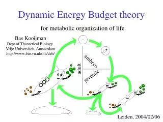
Dynamic Energy Budget theory. 1 Basic Concepts 2 Standard DEB model 3 Metabolism 4 Univariate DEB models 5 Multivariate DEB models 6 Effects of compounds 7 Extensions of DEB models 8 Co-variation of par values 9 Living together 10 Evolution 11 Evaluation.

E N D
Dynamic Energy Budget theory 1 Basic Concepts 2 Standard DEB model 3 Metabolism 4 Univariate DEB models 5 Multivariate DEB models 6 Effects of compounds 7 Extensions of DEB models 8 Co-variation of par values 9 Living together 10 Evolution 11 Evaluation
Body size 3.2 • length: depends on shape and choice (shape coefficient) • volumetric length: cubic root of volume; does not depend on shape • contribution of reserve in lengths is usually small • use of lengths unavoidable because of role of surfaces and volumes • weight: wet, dry, ash-free dry • contribution of reserve in weights can be substantial • easy to measure, but difficult to interpret • C-moles (number of C-atoms as multiple of number of Avogadro) • 1 mol glucose = 6 C-mol glucose • useful for mass balances, but destructive measurement • Problem: with reserve and structure, body size becomes bivariate • We have only indirect access to these quantities
Storage 3.3.2 Plants store water and carbohydrates, Animals frequently store lipids Many reserve materials are less visible specialized Myrmecocystus serve as adipose tissue of the ant colony
Storage 3.3.2a Anthochaera paradoxa (yellow wattlebird) fattens up in autumn to the extent that it can’t fly any longer; Biziura lobata (musk duck) must starve before it can fly
Fractionation from pools & fluxes 3.6b • Examples • uptake of O2, NH3, CO2(phototrophs) • evaporation of H2O • Mechanism • velocity e = ½ m c2 • binding probability to carriers • Examples • anabolic vs catabolic aspects • assimilation, dissipation, growth • Mechanism • binding strength in decomposition
Oxygenic photosynthesis 3.6d CO2 + 2 H2O CH2O + H2O + O2 Reshuffling of 18O Fractionation of 13C
C4 plants 3.6e • Fractionation • weak in C4 plants • strong in C3 plants
Isotopes in products 3.6g • Product flux: fixed fractions of assimilation, dissipation, growth • Assumptions: • no fractionation at separation from source flux • separation is from anabolic sub-flux catabolic flux product flux anabolic flux reserve structure
Change in isotope fractions 3.6h For mixed pool j = E, V (reserve, structure) For non-mixed product j = o (otolith)
Isotopes in biomass & otolith 3.6i body length temperature f,e time, d time, d time, d 0.001 0.001 body length time, d otolith length time, d 0.001 0.001 0.001 opacity otolith length otolith length otolith length otolith length
Flux vs Concentration 3.7 • concept “concentration” implies • spatial homogeneity (at least locally) • biomass of constant composition for intracellular compounds • concept “flux” allows spatial heterogeneity • classic enzyme kinetics relate • production flux to substrate concentration • Synthesizing Unit kinetics relate • production flux to substrate flux • in homogeneous systems: flux conc. (diffusion, convection) • concept “density” resembles “concentration” • but no homogeneous mixing at the molecular level • density = ratio between two amounts
Enzyme kinetics 3.7a Uncatalyzed reaction Enzyme-catalyzed reaction
Synthesizing units 3.7b • Generalized enzymes that process generalized substrates • and follow classic enzyme kinetics • E + S ES EP E + P • with two modifications: • back flux is negligibly small • E + S ES EP E + P • specification of transformation is on the basis of • arrival fluxes of substrates rather than concentrations • In spatially homogeneous environments: • arrival fluxes concentrations
Simultaneous Substrate Processing 3.7c production production Chemical reaction: 1A + 1B 1C Poisson arrival events for molecules A and B blocked time intervals • acceptation event ¤ rejection event Kooijman, 1998 Biophys Chem 73: 179-188
SU kinetics: n1X1+n2X2X3.7d product release product release time 0 tb tc binding prod. cycle Period between subsequent arrivals is exponentially distributed Sum of exponentially distributed vars is gamma distributed Production flux not very sensitive for details of stoichiometry Stoichiometry mainly affects arrival rates
Enzyme kinetics A+BC 3.7.2 Synthesizing Unit Rejection Unit
almost single substr limitation at low conc’s Isoclines for rate A+BC 3.7.2a .2 .6 .8 .2 .4 .6 .8 .4 Conc B Conc A Conc A Rejection Unit Synthesizing Unit
Interactions of substrates 3.7.3 • Substrate interactions in DEB theory are based on Synthesizing Units (SUs): • generalized enzymes that follow the rules of classic enzyme kinetics but • working depends in fluxes of substrates, rather than concentrations • “concentration” only has meaning in homogeneous environments • backward fluxes are small in S + E SE EP E + P • Basic classification • substrates: substitutable vs complementary • processing: sequential vs parellel • Mixture between substitutable & complementary substrates: • grass cow; sheep brains cow; grass + sheep brains cow • Dynamics of SU on the basis of time budgetting • offers framework for foraging theory • example: feeding in Sparus larvae (Lika, Can J Fish & Aquat Sci, 2005): • food searching sequential to mechanic food handling • food processing (digestion) parellel to searching & handling • gives deviations from Holling type II high low low
Interactions of substrates 3.7.3b Kooijman, 2001 Phil Trans R Soc B 356: 331-349
Inhibition 3.7.4 A does not affect B in yACAC; B inhibits binding of A A inhibits binding of B in yACAC; B inhibits binding of A unbounded fraction binding prob of A arrival rate of A dissociation rate of A yield of C on A
Aggressive competition 3.7.4a V structure;E reserve; M maintenance substrate priority E M; posteriority V M JE flux mobilized from reserve specified by DEB theory JV flux mobilized from structure amount of structure (part of maint.) excess returns to structure kV dissociation rate SU-V complex kE dissociation rate SU-E complex kV kE depend on such that kM = yMEkE(E. + EV)+yMVkV .V is constant JEM, JVM kV = kE JEM, JVM kV < kE JE
Social inhibition of x e 3.7.4b sequential parallel substrate conc. No socialization x substrate e reserve y species 1 z species 2 Implications: stable co-existence of competing species “survival of the fittest”? absence of paradox of enrichment biomass conc. dilution rate
Evolution & Co-existence 3.7.4c • Main driving force behind evolution: • Darwin: Survival of the fittest (internal forces) • involves out-competition argument • Wallace: Selection by environment (external forces) • consistent with observed biodiversity • Mean life span of typical species: 5 - 10 Ma • Sub-optimal rare species: • not going extinct soon (“sleeping pool of potential response”) • environmental changes can turn rare into abundant species • Conservation of bio-diversity: • temporal and spatial environmental variation • mutual syntrophic interactions • feeding rates not only depends on food availability (social interaction)
Co-metabolism 3.7.5 Consider coupled transformations A C and B D Binding probability of B to free SU differs from that to SU-A complex
Co-metabolism 3.7.5a binding prob. for substr A
Co-metabolism 3.7.5b Co-metabolic degradation of 3-chloroaniline by Rhodococcus with glucose as primary substrate Data from Schukat et al, 1983 Brandt et al, 2003 Water Research 37, 4843-4854
Co-metabolism 3.7.5c Co-metabolic anearobic degradation of citrate by E. coli with glucose as primary substrate Data from Lütgens and Gottschalk, 1980 Brandt, 2002 PhD thesis VU, Amsterdam
Metabolic modes 3.8.1 CO2 NH3 H2O iron bacterium Gallionella Example of chemolithotrophy 10 H2O O2 4 Fe2+ 4 Fe(OH)3 8 H+ Remember this when you look at your bike/car 4 H2O 4 H2 220 g iron 430 g rust + 1 g bact. 4 Fe
Modules of central metabolism 3.8.2 • Pentose Phosphate (PP) cycle • glucose-6-P ribulose-6-P, • NADP NADPH • Glycolysis • glucose-6-P pyruvate • ADP + P ATP • TriCarboxcyl Acid (TCA) cycle • pyruvate CO2 • NADP NADPH • Respiratory chain • NADPH + O2 NADP + H2O • ADP + P ATP
Central metabolism 3.8.2a • Adenosine Tri-Phosphate (ATP) • 5 106 molecule in 1 bacterial cell • 2 seconds of synthetic work • mean life span: 0.3 seconds
Central Metabolism 3.8.2b source polymers monomers waste/source
Dynamic Energy Budget theory 1 Basic Concepts 2 Standard DEB model 3 Metabolism 4 Univariate DEB models 5 Multivariate DEB models 6 Effects of compounds 7 Extensions of DEB models 8 Co-variation of par values 9 Living together 10 Evolution 11 Evaluation