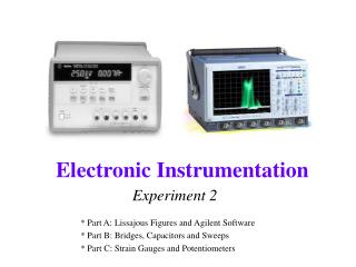
Experiment 2
Experiment 2. * Part A: Intro to Transfer Functions and AC Sweeps * Part B: Phasors, Transfer Functions and Filters * Part C: Using Transfer Functions and RLC Circuits * Part D: Equivalent Impedance and DC Sweeps. Part A. Introduction to Transfer Functions and Phasors

Experiment 2
E N D
Presentation Transcript
Experiment 2 * Part A: Intro to Transfer Functions and AC Sweeps * Part B: Phasors, Transfer Functions and Filters * Part C: Using Transfer Functions and RLC Circuits * Part D: Equivalent Impedance and DC Sweeps
Part A • Introduction to Transfer Functions and Phasors • Complex Polar Coordinates • Complex Impedance (Z) • AC Sweeps
Transfer Functions • The transfer function describes the behavior of a circuit at Vout for all possible Vin.
More Complicated Example What is H now? • H now depends upon the input frequency (w = 2pf) because the capacitor and inductor make the voltages change with the change in current.
How do we model H? • We want a way to combine the effect of the components in terms of their influence on the amplitude and the phase. • We can only do this because the signals are sinusoids • cycle in time • derivatives and integrals are just phase shifts and amplitude changes
We will define Phasors • A phasor is a function of the amplitude and phase of a sinusoidal signal • Phasors allow us to manipulate sinusoids in terms of amplitude and phase changes. • Phasors are based on complex polar coordinates. • Using phasors and complex numbers we will be able to find transfer functions for circuits.
Review of Polar Coordinates point P is at ( rpcosqp , rpsinqp )
Review of Complex Numbers • zp is a single number represented by two numbers • zp has a “real” part (xp) and an “imaginary” part (yp)
Complex Polar Coordinates • z = x+jy where x is A cosf and y is A sinf • wt cycles once around the origin once for each cycle of the sinusoidal wave (w=2pf)
Now we can define Phasors • The real part is our signal. • The two parts allow us to determine the influence of the phase and amplitude changes mathematically. • After we manipulate the numbers, we discard the imaginary part.
The “V=IR” of Phasors • The influence of each component is given by Z, its complex impedance • Once we have Z, we can use phasors to analyze circuits in much the same way that we analyze resistive circuits – except we will be using the complex polar representation.
Magnitude and Phase • Phasors have a magnitude and a phase derived from polar coordinates rules.
Influence of Resistor on Circuit • Resistor modifies the amplitude of the signal by R • Resistor has no effect on the phase
Influence of Inductor on Circuit Note: cosq=sin(q+p/2) • Inductor modifies the amplitude of the signal by wL • Inductor shifts the phase by +p/2
Influence of Capacitor on Circuit • Capacitor modifies the amplitude of the signal by 1/wC • Capacitor shifts the phase by -p/2
Complex Impedance • Z defines the influence of a component on the amplitude and phase of a circuit • Resistors: ZR = R • change the amplitude by R • Capacitors: ZC=1/jwC • change the amplitude by 1/wC • shift the phase -90 (1/j=-j) • Inductors: ZL=jwL • change the amplitude by wL • shift the phase +90 (j)
AC Source sweeps from 1Hz to 10K Hz AC Sweeps Transient at 10 Hz Transient at 100 Hz Transient at 1k Hz
Capture/PSpice Notes • Showing the real and imaginary part of the signal • in Capture: PSpice->Markers->Advanced • ->Real Part of Voltage • ->Imaginary Part of Voltage • in PSpice: Add Trace • real part: R( ) • imaginary part: IMG( ) • Showing the phase of the signal • in Capture: • PSpice->Markers->Advanced->Phase of Voltage • in PSPice: Add Trace • phase: P( )
Part B • Phasors • Complex Transfer Functions • Filters
Definition of a Phasor • The real part is our signal. • The two parts allow us to determine the influence of the phase and amplitude changes mathematically. • After we manipulate the numbers, we discard the imaginary part.
Phasor References • http://ccrma-www.stanford.edu/~jos/filters/Phasor_Notation.html • http://www.ligo.caltech.edu/~vsanni/ph3/ExpACCircuits/ACCircuits.pdf • http://ptolemy.eecs.berkeley.edu/eecs20/berkeley/phasors/demo/phasors.html
Magnitude and Phase • Phasors have a magnitude and a phase derived from polar coordinates rules.
Manipulating Phasors (1) • Note wt is eliminated by the ratio • This gives the phase change between signal 1 and signal 2
Complex Transfer Functions • If we use phasors, we can define H for all circuits in this way. • If we use complex impedances, we can combine all components the way we combine resistors. • H and V are now functions of j and w
Complex Impedance • Z defines the influence of a component on the amplitude and phase of a circuit • Resistors: ZR = R • Capacitors: ZC=1/jwC • Inductors: ZL=jwL • We can use the rules for resistors to analyze circuits with capacitors and inductors if we use phasors and complex impedance.
High and Low Pass Filters High Pass Filter H = 0 at w ® 0 H = 1 at w ®¥ H = 0.707 at wc wc=2pfc fc Low Pass Filter H = 1 at w ® 0 H = 0 at w ®¥ H = 0.707 at wc wc=2pfc fc
Corner Frequency • The corner frequency of an RC or RL circuit tells us where it transitions from low to high or visa versa. • We define it as the place where • For RC circuits: • For RL circuits:
H(jw), wc, and filters • We can use the transfer function, H(jw), and the corner frequency, wc, to easily determine the characteristics of a filter. • If we consider the behavior of the transfer function as w approaches 0 and infinity and look for when H nears 0 and 1, we can identify high and low pass filters. • The corner frequency gives us the point where the filter changes:
Taking limits • At low frequencies, (ie. w=10-3), lowest power of w dominates • At high frequencies (ie. w =10+3), highest power of w dominates
Taking limits -- Example • At low frequencies, (lowest power) • At high frequencies, (highest power)
Our example is a low pass filter What about the phase?
Part C • Using Transfer Functions • Capacitor Impedance Proof • More Filters • Transfer Functions of RLC Circuits
Capacitor Impedance Proof Prove:
Band Filters Band Pass Filter H = 0 at w ® 0 H = 0 at w ®¥ H = 1 at w0=2pf0 f0 Band Reject Filter H = 1 at w ® 0 H = 1 at w ®¥ H = 0 at w0 =2pf0 f0
Resonant Frequency • The resonant frequency of an RLC circuit tells us where it reaches a maximum or minimum. • This can define the center of the band (on a band filter) or the location of the transition (on a high or low pass filter). • The equation for the resonant frequency of an RLC circuit is: