Download
1 / 20
200 likes | 474 Views
GPU Nearest Neighbor Searches using a Minimal kd-tree. Shawn Brown. Jack Snoeyink. Department of Computer Science University of North Carolina at Chapel Hill. s hawndb@cs.unc.edu. snoeyink @cs.unc.edu. Goal: Write spatial streaming tool to process

E N D
GPU Nearest Neighbor Searches using a Minimal kd-tree Shawn Brown Jack Snoeyink Department of Computer Science University of North Carolina at Chapel Hill shawndb@cs.unc.edu snoeyink@cs.unc.edu Goal: Write spatial streaming tool to process billions of points by applying operators to local neighborhoods.
NN Search Types • Definitions: • d, number of dimensions • S is a search set containing ‘n’ points • Q is a query set containing ‘m’ points • dist(a,b) is a distance metric between two points QNN: Query Nearest Neighbor Find the closest point in S for each point in Q bydist(p,q). Input:S, Q Output:List of m indices of closest points in S. All-NN: All Nearest Neighbor Find the closest point in S for each point in Sbydist(p,q). Input:S (Q ↔ S) Output:List of n indices in S. Note: Exclude zero distance results kNN: ‘k’ Nearest Neighbors Find the k closest points in S for each point in Q bydist(p,q). Input:S, Q Output:List of km indices of closest points in S. All-kNN: All‘k’ Nearest Neighbors Find the k closest points in S for each point in Sbydist(p,q). Input:S(Q↔ S) Output:List of km indices in S. Note: Exclude zero distance results RNN: Range Query ANN: Approximate Nearest Neighbor
NN search Solutions Linear Search: Brute force solution, compare each query point to all search points O(mn) Spatial Partitioning Data Structures: Divide space into smaller spatial cells.Use “branch and bound” to focus on productive cells. Examples: kd-tree, Quad-tree, Grid, Voronoi Diagram, … Spatial Partitioning: subdivide space Data Partitioning: subdivide data into sets
NN Searches on GPU • Zhou 2008 • Breadth first search kd-tree • Voxel Volume split heuristic • Build time: 9-13x faster vs. CPU • Search time:7-10x faster vs. CPU • Qiu 2008 • Depth first search kd-tree • Median split heuristic • Approximate • Registration time: 100x faster vs. CPU • Purcell 2003 • Multi-pass using uniform grid • Approximate • Bustos 2006 • Trick video card into finding Manhattan distance by texture operations • Rozen 2008 • Bucket points into 3D cells then brute force search on 3x3x3 neighborhoods • Garcia 2008 • Brute force algorithm Search time: 100x faster vs. MATLAB
kd-tree • Invented by J.L. Bentley, 1975 • Spatial partitioning data structure • Hierarchical • Supports d-dimensional points and more complicated objects • Made up of axis aligned spatial cells • Root cell corresponds to original bounds and contains all points • Each spatial cell also corresponds to a node of a binary tree. • Recursively defined by dividing each cell into a left and right cell starting from the root. • Points associated with each cell are also partitioned into the left and right child cells • Splitting Heuristics • For each node of the binary tree • Form a cutting plane (pick an axis and split value) • Pick cutting plane via a splitting heuristic • Median split, empty space maximization, surface area, voxel volume, etc.
Building a kd-tree Add root cell to build queue While build queue not empty • Pop current cell from build queue • Pick cutting plane from median split • build left & right child cells • Partition points into left & right cells • Add left & right child to build queue Storage: O(dn) Build Time: O(dn log n) • More Details: • Build kd-tree on CPU, transfer kd-nodes to GPU • Median Split → use Quickmedian selection algorithm • Build a remap array → converts node indices into point indices
Trim Test Onside Offside Searching a kd-tree ** Based on Arya’s Efficient NN kd-tree Method Push root node onto stack Recursively search children** • Pop current search node off stack • Trim Test current node, if offside • currDist = dist(qp, currNode.point), • Update Best distance, if currDist is closer • Map left/right nodes ontoonside/offside • Trim Test& Push offside node onto stack • Push onside node →Point Location NN = Best distance (Best index) Search Times Best: Expected: Worst: • Onside = child cell with query Offside= leftover child cell. • No 1D overlap → safe to discard the entire sub-tree.
GTX 285 Architecture SIMD Thread Processor GPU Device • Device Resources • 30 GPU Cores • 240 total thread processors • 1 GB on-board RAM • 32 KB constant memory • GPU Core • 8 Thread processers per core • 1 double precision unit per core • 16 KB shared memory • 8,192 shared 32-bit registers • Thread Processor • Shares resources (memory, registers) in same core GPU Core Double Shared Memory
Execution Model Hardware Software Notes Thread Processor Threads are executed by thread processors Thread • Threads blocks executed on GPU cores • Thread blocks start & stay with initial core • Thread block finishes when all threads finish • Multiple blocks get mapped to each core • One GPU core can execute several blocks concurrently depending on resources • Syncing of threads within a block • Maximum of 512 threads per thread block GPU Core Thread Block GPU Device Grid A kernel is launched as a 2D or 1D Grid of thread blocks Only one kernel can execute on a GPU device at a time. Syncing across blocks not supported
GPU Hardware Limits and Design Choices • Floats (IEEE 754 compliant) • focus on singles (32-bit) • doubles (64-bit) →8x slower • Memory • Aligned data (4,8,16 bytes) → better performance • limited capacity → use minimal data structures • Memory Hierarchyregisters » shared » constant » RAM • Local variables → registers • Structures/arrays → shared • Thread Block Size • 4-16 threads per block is optimal based on testing • Latency • Hide I/O latency by massive scheduling of threads • 1 thread per query point • Divergence • Divergent branching degrades performance → Minimize branching • Coalesence GPU can coalesce aligned sequential I/O requests Unfortunately, kd-tree doesn’t result in aligned I/O requests Good = 1 I/O op Bad = 16 I/O ops Aligned, Sequential
kd-tree Design Choices • Bound kd-tree Height • Bound height to ceil[log2n] • Build a balanced static kd-tree • Store as left-balanced binary array • Minimal Foot-print • Store one point per node O(dn) • Eliminate fields • No pointers (parent, child) → Compute directly • No cell min/max bounds • Single split plane per cell is sufficient • Split plane (value, axis) is implicit • Cyclickd-tree axis access → track via stack • kd-tree →inplacereorder of search points • Final kd-tree Design: • Static • Balanced • Median Split • Minimal (Inplace) • Cyclic • Storage: • one point per node • left balanced array
Left Balanced Median (LBM) h = log2(n+1) half = 2h-2 lastRow = n – (2•half)+ 1 LBM = half +min(half,lastRow) Left Balanced Tree / Array Parent Curr … Root Left Right … Last … i/2 i 1 2i 2i+1 n n+1 2h-1 Links: Given node @ i Parent = i/2 Left = 2i Right = 2i+1 Tests: isRoot (i==1) isInvalid(i> n) isLeaf(2i > n) & ((2i+1)>n)
Optimal Thread Block Size QNN, All-NN The Optimal thread block Is 10x1 for n,m=1 million points kNN, All-kNN The optimal thread block size is 4x1 for n,m=1 million points, k=31
Increasing n,m; Increasing k Increasing n,m; n ≤ 100, use CPU n ≥1000, use GPU Increasing k (kNN, All- kNN) Divergence on GPU gradually hurts performance
ResultsGPU: GTX 285 using CUDA 2.3CPU: Intel I7-920 @ 2.4Ghz • 2D Results: NN up to 36 million pointskNN up to 1 million, k=31on GPU • QNN: GPU runs 20-44x faster than CPU • All-NN: GPU runs 10-40x faster than CPU • kNN: GPU runs 13-18x faster than CPU • All-kNN: GPU runs 8-17x faster than CPU • 3D & 4D Results: NN up to 22 million points kNN1 million, k=31 on GPU • 3D: Runs 7-29x faster than CPU. • 4D: Runs 6-22x faster than CPU.
Future Directions • Streaming Neighborhood Tool • Apply operators on local neighborhoods (billions of points) • Build on GPU • 1st Attempt: works correctly but is slower than CPU solution • Improve coalescence, Increase # of threads • Compare against other solutions • CGAL, GPU Quadtree, GPU Morton Z-order sort • Improve Search performance • Store top 5-10 levels of tree in constant memory • All-NN, All-kNN rewrite search to be bottom-up • Improve code • Use ‘Templates’ to reduce total amount of code • Move code to other APIs / Platforms • OpenMP • OpenCL • ATI Stream
Thank You • Any Questions ? The paper, more detailed results, & the source code are stored at … http://cs.unc.edu/~shawndb/
Appendix A:CPU Host Scaffolding • Computes Thread Block Grid Layout • Pads n,m to block grid layout • Allocates memory resources • Initializes search, query lists • Builds kd-tree • Transfers inputs onto GPU • kd-tree, search, query data • Invokes GPU Kernel • Transfers NN results back onto CPU • Validates GPU results against CPU search, • if requested • Cleanup memory resources
Appendix B:Minimal Data Structures // GPU Point (3D) → 16 bytes typedefstruct__align__(16) { float pos[3]; // Point <x,y,z> } GPU_Point3D; // GPU Search Item → 8 bytes typedefstruct__align__(8) { unsigned intnodeFlags; // Below float splitVal; // Split Value } GPU_Search; // GPU kd-node (3D) → 16 bytes typedefstruct__align__(16) { float pos[3]; // Point <x,y,z> } GPUNode_3D_LBT; nodeFlags // 3 fields compressed into 32 bits Node Index[0..27] // 2^28 points max. in kd-tree. Split Axis[28..30] // 2^3 = 8d points max. OnOff[31] // Onside/offside status // NN Result → 8 bytes typedefstruct__align__(8) { unsigned int Id; // Best ID float Dist; // Best Distance } GPU_NN_Result;
Appendix C: More Search Details • Cyclic • start at root with x-axis • nextAxis = (currAxis + 1) % d; prevAxis = (currAxis – 1) % d; • Backtrack via DFS stack, not BFS queue • Less storage→ shared memory: O(log n) stack vs. O(n) queue • Better trim behavior: 40-80 iterations using stack vs. 200-500 iterations using queue • 12 GPU kernels • NN types (QNN, All-NN, kNN, All-kNN) * (2D,3D,4D) = 12 kernels • One thread per query point • I/O Latency overcome through thread scheduling • Thread block must wait on slowest thread to finish • Avoid slow I/O operations (RAM) • 1 I/O (load point) per search loop • extra trim test → continue loop before doing unnecessary I/O • Remap once from node index to point index at end of search • kNN search • Closest heap data structure • Acts like array (k-1 inserts) then acts like max-heap • Trim distance kept equal to top of heap