Download
1 / 35
350 likes | 376 Views
Learn about the business cycle, short run vs long run, aggregate demand and supply, and analyzing the effects of shocks on the economy.

E N D
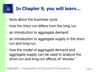
In Chapter 9, you will learn… • facts about the business cycle • how the short run differs from the long run • an introduction to aggregate demand • an introduction to aggregate supply in the short run and long run • how the model of aggregate demand and aggregate supply can be used to analyze the short-run and long-run effects of “shocks.” CHAPTER 9 Introduction to Economic Fluctuations
Facts about the business cycle • GDP growth averages 3–3.5 percent per year over the long run with large fluctuations in the short run. • Consumption and investment fluctuate with GDP, but consumption tends to be less volatile and investment more volatile than GDP. • Unemployment rises during recessions and falls during expansions. • Okun’s Law: the negative relationship between GDP and unemployment. CHAPTER 9 Introduction to Economic Fluctuations
Real GDP growth rate Investment growth rate Consumption growth rate Growth rates of real GDP, consumption, investment Percent change from 4 quarters earlier 40 30 20 10 0 -10 -20 -30 1970 1975 1980 1985 1990 1995 2000 2005
1970 1975 1980 1985 1990 1995 2000 2005 Unemployment Percent of labor force 12 10 8 6 4 2 0
1966 1951 1984 2003 1987 1975 2001 1982 1991 -3 -2 -1 0 1 2 3 4 Okun’s Law 10 Percentage change in real GDP 8 6 4 2 0 -2 -4 Change in unemployment rate
Index of Leading Economic Indicators • Published monthly by the Conference Board. • Aims to forecast changes in economic activity 6-9 months into the future. • Used in planning by businesses and govt, despite not being a perfect predictor. CHAPTER 9 Introduction to Economic Fluctuations
Components of the LEI index • Average workweek in manufacturing • Initial weekly claims for unemployment insurance • New orders for consumer goods and materials • New orders, nondefense capital goods • Vendor performance • New building permits issued • Index of stock prices • M2 • Yield spread (10-year minus 3-month) on Treasuries • Index of consumer expectations CHAPTER 9 Introduction to Economic Fluctuations
Index of Leading Economic Indicators 160 140 120 100 1996 = 100 80 60 40 20 0 Source: Conference Board 1970 1975 1980 1985 1990 1995 2000 2005
Time horizons in macroeconomics • Long run: Prices are flexible, respond to changes in supply or demand. • Short run:Many prices are “sticky” at some predetermined level. The economy behaves much differently when prices are sticky. CHAPTER 9 Introduction to Economic Fluctuations
Recap of classical macro theory (Chaps. 3-8) • Output is determined by the supply side: • supplies of capital, labor • technology. • Changes in demand for goods & services (C, I, G ) only affect prices, not quantities. • Assumes complete price flexibility. • Applies to the long run. CHAPTER 9 Introduction to Economic Fluctuations
When prices are sticky… …output and employment also depend on demand, which is affected by • fiscal policy (G and T ) • monetary policy (M ) • other factors, like exogenous changes in C or I. CHAPTER 9 Introduction to Economic Fluctuations
The model of aggregate demand and supply • the paradigm most mainstream economists and policymakers use to think about economic fluctuations and policies to stabilize the economy • shows how the price level and aggregate output are determined • shows how the economy’s behavior is different in the short run and long run CHAPTER 9 Introduction to Economic Fluctuations
Aggregate demand • The aggregate demand curve shows the relationship between the price level and the quantity of output demanded. • For this chapter’s intro to the AD/AS model, we use a simple theory of aggregate demand based on the quantity theory of money. • Chapters 10-12 develop the theory of aggregate demand in more detail. CHAPTER 9 Introduction to Economic Fluctuations
The Quantity Equation as Aggregate Demand • From Chapter 4, recall the quantity equation M V = P Y • For given values of M and V, this equation implies an inverse relationship between P and Y: CHAPTER 9 Introduction to Economic Fluctuations
P AD Y The downward-sloping AD curve An increase in the price level causes a fall in real money balances (M/P), causing a decrease in the demand for goods & services. CHAPTER 9 Introduction to Economic Fluctuations
P AD2 AD1 Y Shifting the AD curve An increase in the money supply shifts the AD curve to the right. CHAPTER 9 Introduction to Economic Fluctuations
Aggregate supply in the long run • Recall from Chapter 3: In the long run, output is determined by factor supplies and technology is the full-employment or natural level of output, the level of output at which the economy’s resources are fully employed. “Full employment” means that unemployment equals its natural rate (not zero). CHAPTER 9 Introduction to Economic Fluctuations
LRAS P Y The long-run aggregate supply curve does not depend on P, so LRAS is vertical. CHAPTER 9 Introduction to Economic Fluctuations
LRAS P P2 In the long run, this raises the price level… AD2 AD1 Y …but leaves output the same. Long-run effects of an increase in M An increase in M shifts AD to the right. P1 CHAPTER 9 Introduction to Economic Fluctuations
Aggregate supply in the short run • Many prices are sticky in the short run. • For now (and through Chap. 12), we assume • all prices are stuck at a predetermined level in the short run. • firms are willing to sell as much at that price level as their customers are willing to buy. • Therefore, the short-run aggregate supply (SRAS) curve is horizontal: CHAPTER 9 Introduction to Economic Fluctuations
The SRAS curve is horizontal: The price level is fixed at a predetermined level, and firms sell as much as buyers demand. P SRAS Y The short-run aggregate supply curve CHAPTER 9 Introduction to Economic Fluctuations
In the short run when prices are sticky,… P SRAS AD2 AD1 Y …causes output to rise. Y2 Short-run effects of an increase in M …an increase in aggregate demand… Y1 CHAPTER 9 Introduction to Economic Fluctuations
From the short run to the long run Over time, prices gradually become “unstuck.” When they do, will they rise or fall? In the short-run equilibrium, if then over time, P will… rise fall remain constant The adjustment of prices is what moves the economy to its long-run equilibrium. CHAPTER 9 Introduction to Economic Fluctuations
LRAS P P2 SRAS AD2 AD1 Y Y2 The SR & LR effects of M>0 A = initial equilibrium B = new short-run eq’m after Fed increases M C B A C = long-run equilibrium CHAPTER 9 Introduction to Economic Fluctuations
How shocking!!! • shocks: exogenous changes in agg. supply or demand • Shocks temporarily push the economy away from full employment. • Example: exogenous decrease in velocity If the money supply is held constant, a decrease in V means people will be using their money in fewer transactions, causing a decrease in demand for goods and services. CHAPTER 9 Introduction to Economic Fluctuations
AD shifts left, depressing output and employment in the short run. LRAS P P2 SRAS AD2 AD1 Y Y2 The effects of a negative demand shock A B Over time, prices fall and the economy moves down its demand curve toward full-employment. C CHAPTER 9 Introduction to Economic Fluctuations
Supply shocks • A supply shock alters production costs, affects the prices that firms charge. (also called price shocks) • Examples of adverse supply shocks: • Bad weather reduces crop yields, pushing up food prices. • Workers unionize, negotiate wage increases. • New environmental regulations require firms to reduce emissions. Firms charge higher prices to help cover the costs of compliance. • Favorable supply shocks lower costs and prices. CHAPTER 9 Introduction to Economic Fluctuations
CASE STUDY: The 1970s oil shocks • Early 1970s: OPEC coordinates a reduction in the supply of oil. • Oil prices rose 11% in 1973 68% in 1974 16% in 1975 • Such sharp oil price increases are supply shocks because they significantly impact production costs and prices. CHAPTER 9 Introduction to Economic Fluctuations
The oil price shock shifts SRAS up, causing output and employment to fall. LRAS P SRAS2 SRAS1 AD Y Y2 CASE STUDY: The 1970s oil shocks B In absence of further price shocks, prices will fall over time and economy moves back toward full employment. A A CHAPTER 9 Introduction to Economic Fluctuations
Stabilization policy • definition: policy actions aimed at reducing the severity of short-run economic fluctuations. • Example: Using monetary policy to combat the effects of adverse supply shocks: CHAPTER 9 Introduction to Economic Fluctuations
LRAS P SRAS2 SRAS1 AD1 Y Y2 Stabilizing output with monetary policy The adverse supply shock moves the economy to point B. B A CHAPTER 9 Introduction to Economic Fluctuations
LRAS P SRAS2 AD2 AD1 Y Y2 Stabilizing output with monetary policy But the B of C accommodates the shock by raising agg. demand. B C A results: P is permanently higher, but Y remains at its full-employment level. CHAPTER 9 Introduction to Economic Fluctuations
Chapter Summary 1. Long run: prices are flexible, output and employment are always at their natural rates, and the classical theory applies. Short run: prices are sticky, shocks can push output and employment away from their natural rates. 2. Aggregate demand and supply: a framework to analyze economic fluctuations CHAPTER 9 Introduction to Economic Fluctuations slide 32
Chapter Summary 3. The aggregate demand curve slopes downward. 4. The long-run aggregate supply curve is vertical, because output depends on technology and factor supplies, but not prices. 5. The short-run aggregate supply curve is horizontal, because prices are sticky at predetermined levels. CHAPTER 9 Introduction to Economic Fluctuations slide 33
Chapter Summary 6. Shocks to aggregate demand and supply cause fluctuations in GDP and employment in the short run. 7. The B of C can attempt to stabilize the economy with monetary policy. CHAPTER 9 Introduction to Economic Fluctuations slide 34