Download
1 / 27
270 likes | 281 Views
Explore the process of recovering vocal tract shape from acoustic signals through innovative inversion techniques, benefitting speech research and technology applications.

E N D
Acoustic to articulatory inversion of speech Yves Laprie Speech Group INRIA Lorraine
Layout • Introduction • Our approach • The table lookup procedure • Construction of the hypercube table • Inversion with the hypercube table • Recovering articulatory trajectories • Experiments
What is acoustic to articulatory inversion ? Recovering the temporal evolution of the vocal tract shape from the acoustic signal. Acoustical signal represented by the three first resonance frequencies (formants). The vocal tract shape is given by seven articulatory parameters (jaw, tongue position and shape, apex, lip aperture and protrusion and larynx). These parameters correspond to the articulatory model of Maeda.
Why is inversion useful ? Theoretical interests: • A better knowledge of speech production • A better comprehension of audio-visual integration Applicative interests: • Very low bit rate speech coding • Automatic speech recognition • A feedback for language learning
Why inversion is difficult? There is no one-to-one mapping between vocal tract shapes and speech spectra (recovering more articulatory parameters than acoustic parameters measured from speech). An analysis by synthesis method to limit the space of inverse solutions. Articulatory parameters saggital slice Area function Speech spectrum Model of saggital to area transformation Acoustic simulation: Acoustic/electrical analogy (acoustic tubes –electrical quadripoles) Articulatory model inversion
How the vocal tract can be represented ? • Two extreme solutions: • A drastically simplified representation of the vocal tract (e.g. 6 uniform tubes). • does not ensure that the evolution of the vocal tract shape is realistic. • A more realistic 3D representation of the vocal tract obtained by PCA methods applied to MRI images. • how constraints consistent with the vocal tract dynamics can be incorporated in the inversion ?
Layout • Introduction • Our approach • The table lookup procedure • Construction of the hypercube table • Inversion with the hypercube table • Recovering articulatory trajectories • Experiments
Our position We want to interpret inversion results in terms of articulator movements, so that a phonetic representation of sounds can be exploited later. Articulatory model (that of Maeda) We want to prevent the inversion method from influencing inversion results implicitly. An inversion method as neutral as possible (keep all the inverse solutions). Adding constraints or a learning phase to study their influence on the inversion.
Our approach • A table lookup procedure to find inverse solutions at each time of the speech signal to be inversed. • An exploration algorithm to build articulatory trajectories along the time interval of the speech signal. • A regularization method to improve the regularity of articulatory trajectories as well as their acoustic proximity with acoustical data.
Layout • Introduction • Our approach • The table lookup procedure • Construction of the hypercube table • Inversion with the hypercube table • Recovering articulatory trajectories • Experiments
Articulatory synthesizer • Application f: A Ac • A articulatory space • Ac acoustic space Articulatory parameters chosen according to some criterion Acoustical parameters N M N M Table Articulatory parameters indexed by acoustical parameters Table lookup procedure Requires the construction of an articulatory table. Difficulties: The dimension of the articulatory space is 7. The articulatory to acoustic mapping is not linear.
Some methods for constructing articulatory tables • Regularly spaced sampling • Seven parameters, each of them varies between -3 and +3 ! • Random sampling tables • A (very) limited number of shapes without any control on the location of the articulatory parameters in the articulatory space. • Random sampling in the vicinity of paths between two root shapes corresponding to vowels • Requires very consistent root shapes in terms of articulatory parameters.
A hypercubic articulatory table Adaptative sampling of the articulatory space to account for non-linearities of the articulatory-to-acoustic mapping denoted ℳ. Construction: • The articulary space is included in a 7 dimensional root hypercube. • If the mapping ℳ is not linear inside this hypercube, this hypercube is subdivided into (27 = 128) sub-hypercubes. • A hypercube is kept only if the mapping is sufficiently linear. • The table is a hierarchy of hypercubes.
Linearity evaluation in a 3 dimesional hypercube. Comparing formant values (acoustical parameters) interpolated against those calculated by synthesis.
Experimental evaluation of the interpolation accuracy • Comparing formant values interpolated from the hypercubes with those synthesized for 2000 random articulatory points. • We get a better precision than that imposed during hypercube construction.
Layout • Introduction • Our approach • The table lookup procedure • Construction of the hypercube table • Inversion with the hypercube table • Recovering articulatory trajectories • Experiments
Inversion based on the hypercube table • For one acoustic vector (3-tuple of formants F1, F2 and F3) at a time : • finding all the hypercubes whose acoustical images given by the mapping ℳ contain the 3-tuple of formants. • finding all the inverse solutions in each of these hypercubes. Formant vector measured Formant vector at P0 Hypercube center Jacobian of ℳ Inverse points More unknowns (7) than know data (3).
Sampling the intersection of the null space of F and the hypercube Hc (1) SVD provides a particular solution (Psvd) plus a basis of the null space (a 4 dimensional space for F). (Null space of F) Each P must belong to Hc, i.e. for each coordinate i : and are the lower and higher boundaries of the ith coordinate of the hypercube.
Sampling the intersection of the null space of F and the hypercube Hc (2) • There is no exact solution of the problem beyond dimension 3. • Linear programming to find lower and higher values of j (4 programs for the lower values and 4 for the higher values). • Regular sampling the jand verifying that the corresponding points belong to the hypercube. Sampling of the null space Intersection with the hypercube
Layout • Introduction • Our approach • The table lookup procedure • Construction of the hypercube table • Inversion with the hypercube table • Recovering articulatory trajectories • Experiments
? Standard deviation of one of the articulatory parameters Time Recovering articulatory trajectories /ui/ – All the inverse solutions for the /ui/ speech signal with a 30Hz precision for the three first formants.
Recovering articulatory trajectories • A method which operates in two steps: • A dynamic programming that minimizes articulatory efforts along articulatory trajectories. • A regularizing method that incorporates the acoustic behavior of the articulatory model and uses solutions of step 1 as initial solutions. • Two criteria are combined : • acoustical proximity between original and synthesized formants. • Regularity of articulatory trajectories.
Layout • Introduction • Our approach • The table lookup procedure • Construction of the hypercube table • Inversion with the hypercube table • Recovering articulatory trajectories • Experiments
Experiments Transition /yi/ F3 F2 F1 F3 Re-synthesized vs. original formants Frequency (Hz) F2 F1 Time (ms)
Inverse articulatory trajectories With a constraint on the protrusion of the first point. With a constraint on the protrusion and the jaw of the first point. Without any constraint
Comparison of the vocal tract shapes Both solutions produce exactly the same formants, i.e. the same acoustical signal. Only the strategy for exploiting acoustical properties of the articulatory model differ. Without any constraint. With a constraint on the protrusion and the jaw of the first point.
Conclusions • All the inverse solutions are potentially explored, i.e. the inversion procedure does not influence solutions. • The accuracy of inversion can be decreased so that errors on the model adaptation do not influence inversion. • Learning probabilities of articulatory shapes from real data to guide inversion towards articulatory trajectories realized by real speakers. • Audio-visual inversion: Incorporating constraints through the recovering of visible articulators (jaw and lips) to reduce the dimension of the solution space.