Algorithmics and Complexity
Delve into the limits of solvability with algorithms and the concept of efficiency measurement. Explore the undecidable Halting Problem paradox and assess algorithm efficiency across time and storage space. Learn key questions and measures in algorithmic complexity.

Algorithmics and Complexity
E N D
Presentation Transcript
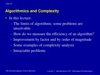
Algorithmics and Complexity • In this lecture: • The limits of algorithms: some problems are unsolvable. • How do we measure the efficiency of an algorithm? • Improvement by factor and by order of magnitude • Some examples of complexity analysis • Intractable problems
Can Computers Solve Every Problem? • It seems that computers are powerful enough as to enable us to solve any problem by writing the appropriate program. • It may (or may not) seem quite surprising to know, that there are problems which cannot be solved by any computer! • Such problems were discovered and studied by the mathematician Alan Turing, the most famous of which is the Halting Problem (1937).
The Halting Problem • Given a program P and an input x, does the program P halt on the input x? • One can imagine a method booelan doesHalt(P,x) that does the following: • reads the program P (which is just a text file) • runs an algorithm which determines if the program P halts on the input x • returns true if P halts on the specified input x • returns false if P does not halt on the specified input x
The Halting Problem • Define a program: testHalt(P) { if (doesHalt(P,P)) loop forever; else print “halt”; } • What happens if we run testHalt, and give it as input testHalt itself? testHalt(testHalt)
The Halting Problem Paradox • Assume testHalt(testHalt) terminates and prints “halt”: • This means doesHalt(testHalt,testHalt) returned false, which in turn means that testHaltdoes not terminate on the input testHalt! A contradiction! • Assume testHalt(testHalt) loops forever: • This means doesHalt(testHalt,testHalt) returned true, which in turn means that testHaltdoes terminate on the input testHalt! Another contradiction! • Conclusion: Our assumption, that there exists a method doesHalt, which determines if a program halts on a specific input, is wrong! • In computer science terms, We say that the Halting Problem is undecidable. (בלתי כריעה).
Halting Problem - The Bright Side • We have proved that no algorithm can solve the halting problem. • In contrast to the halting problem, we have already seen that: • there are problems which can be solved algorithmically • There may be more than one way to solve a particular problem (sorting).
Algorithmic Questions • When we are given a specific problem, there are many questions we can ask about it: • Are there algorithms which solve this problem? (חישוביות) • Given an algorithm which solves the problem, how can we be convinced that the algorithm is correct? • How good is an algorithm which solves the problem? • Is it efficient in terms of processing steps (time)? • Is it efficient in terms of storage space (memory)? • How do we measure efficiency? (סיבוכיות)
More Algorithmic Questions • More questions we can ask: • Is there something we can say about every algorithm which solves the problem? • For example, every algorithm must take at least x processing steps, etc… • When we implement the algorithm on a computer, will the problem be solved within a reasonable time? What is reasonable, anyway? • Phone lookup (144) - few seconds • Weather forecast - max. one day • Cruise missiles - real time (a late answer is useless…) • Physical simulations - few days? Few weeks? Perhaps more?
Time Efficiency • How do we measure time efficiency? • Assume we have a problem P to solve, with two algorithms A1 and A2 that solve it. • We wish to compare A1 and A2’s efficiency. • What do you think about the following efficiency test? • The algorithms were implemented on a computer, and their running time was measured: • Algorithm A1 - 1.25 seconds • Algorithm A2 - 0.34 seconds • Conclusion: Algorithm A2 is better!
Time Efficiency: Questions We Must Ask • Were the algorithms tested on the same computer? • Is there a “benchmark” computer on which we test algorithms? • What were the inputs given to the algorithm? Were the inputs equal? Of equal size? • Is there a better way for measuring time efficiency, independent of a particular computer?
Input Size • The running time of an algorithm is dependent upon the “amount of work” is has to perform, which in turn is a function of the size of input given to the algorithm: • In an array sorting algorithm - number of cells to sort • In an algorithm for finding a word in a text - number of characters, or number of words • In an algorithm that tests if a number is prime: size of number (number of bits which represent the number, or number of digits)
Efficiency Measure - First Attempt • A reasonable way to measure the time efficiency of an algorithm could be: • find out how many “steps” the algorithm performs for every input size (= as a function of the input size). • What could those “steps” be? • Anything we find reasonable, as long as we know those “steps” take approximately “constant” time to run, that is, their running time is not a function of the input size
Algorithmic Steps Examples • In the bubble sort algorithm: switch two adjacent cells. • In a “generic” algorithm for finding an element in an array: • Do until stop: • Find out what is the next cell to look at (or stop) • Find out if the element we’re looking for is in this cell • In an algorithm for testing if a number x is prime: find out if y divides x. • In a classic algorithm for multiplying two numbers: multiply digits / add digits. • Note that all these steps take “constant” time to perform, which is not dependent upon the size of input.
Advantages of the Suggested Measurement • It is not dependent on a particular computer. • If we wish to figure out what will be the running time of the algorithm on a particular computer, we’ll just have to: • Estimate how long does it take to perform the “basic steps” we’ve defined on the particular computer • multiply this measurement by the number of steps we’ve calculated for a specific input size.
Example: Character Search • Problem: Find out if the character c occurs in a given text. • Solution 1 • found false • while (more characters to read and found == false) • read the next character in the text • if this character is c, found true. • If (end of text reached) print (“not found”) else print(“found”).
Solution 1 Time Analysis • Input size? • Number of characters in text • What is the basic step? • Find out if end of text has been reached • read next character in text • Test if character is c; • What is the running time as function of input length n? • Depends on the particular text. But, in the worse case, no more than n basic steps + constant (operations before and after loop). • T(n) <= c1n + d1
Character Search: Simple Optimization • Solution 2 • found false; • add c to end of text • while (found == false) • read the next character in the text • if this character is c, found true. • If (end of text reached) print (“not found”) else print(“found”). • Remove c from end of text.
Solution 2 Time Analysis • Solution 2 analysis is more or less the same, however the basic step is different: • read next character in text • Test if character is c • In the worse case, the running time of Solution 2 as a function of n is • T(n) <= c2n + d2 • This time, c2 and d2 are different. (c1 > c2 , d2 > d1). • In solution 2, we have: • shortened the time it takes to perform the basic step, but: • added a constant to the overall running time
Running Time Tables Input Size 1 3 5 10 100 1000 30000 3000000 3n + 2 5 11 17 32 302 3002 90002 9000002 2n + 4 6 10 14 24 204 2004 60004 6000004 ratio 0.83 1.1 1.21 1.33 1.48 ~1.5 ~1.5 ~1.5
Improvement by Factor • In short texts, Solution 1 is better than Solution 2 (the improved solution), however: • As the text length grows, the constants d1 and d2 become less and less important, and the ratio converges to 1.5. • Such improvement is called an improvement by factor, since the ratio between the running times of both solutions, as n grows, converges to a constant.
A Word about Best, Average and Worse cases • Note that when we have counted the number of steps, we have analyzed the worse case, in which the character c is not in the text. • Other measurement: Average case. • What is the advantage of measuring the worse case? • The average case is a good measurement, however, for a specific input length n, we have no idea what the running time will be. • Computing the average case is quite complex. • What information does Best Case analysis give us?
Improvement by Factor: Is it Important? • We shall soon see that many times we can do better than improving the running time by a factor • However, improvement by factor is still important: • If we make an effort at optimizing specific “bottleneck” areas in a program, we may gain a lot • Special programs called profilers help us in pinpointing the “hot” areas in a program. The 80/20 rule (or 90/10 rule): A program spends 80% of its time executing 20% of its code.
Finding a Phone Number in a Phonebook • Problem: Find if a number x appears in a sorted array of numbers (e.g., a phonebook). • This problem is similar to the character search problem. • The algorithms we have already seen can be used to solve this problem: both algorithms are quite similar, and are a variant of the serial search method. • [Other possible optimizations?] • However, the assumption that the array is sorted can be used in a clever way.
Binary Search • “Cut out” half of the search space in every step. • The basic step in binary search: • Find out if the current cell contains the number we’re looking for • Termination condition: find out if the range is of size 1 • If 1 and 2 is false, calculate the next cell to look for (index = middle cell in current range) • The basic step in serial search: • Find out if the current cell contains the number we’re looking for • Termination condition: find out if we have reached the end of array • If 1 and 2 is false, calculate the next cell to look for (index = index + 1)
Binary Search - Example • If the array is of size 1000, in the worse case, we will be looking at ranges of size 1000,500,250,125,63,32,16,8,4,2,1, total of 10 steps. • Compare to serial search: 1000 steps! • With million cells, we will be looking at 20 cells in the worse case • How many cells in the general case?
Binary vs. Serial - Number of Steps Input Size 10 100 1000 10000 100000 1000000 serial 10 100 1000 10000 100000 1000000 binary 4 7 10 14 17 20 ratio ~2.5 ~14 ~100 ~714 ~5883 ~50000
Improvement by Order of Magnitude • Recall, that when we have dealt with improvement in factor, the ratio between running times was constant. • This time, we can evidently see the the ratio between the number of steps is growing as the input size grows. • This kind of improvement is called improvement by order of magnitude.
What About the Duration of Basic Step? • When we have dealt with improvement in factor, the duration of a basic step was very interesting. • Is it of importance now? • Or, put in other words: Assume that the duration of a single step in serial search is 1 and that a single step in binary search takes 1000, would there still be an improvement?
Binary vs. Serail - Different Duration of Steps Input Size 10 100 1000 10000 100000 1000000 serial 10 100 1000 10000 100000 1000000 binary 400 700 1000 1400 1700 2000 ratio ~0.025 ~0.14 1 ~7.14 ~58.8 ~500
Duration of Basic Step is Negligible • As we can see from the table, for small input sizes ( < 1000), serial search is indeed better • However, for larger input sizes, binary search still wins. • The reason is very simple: the ratio between duration of basic steps is constant, while the ratio between the number of basic steps grows as the input size grows. • Note that in practice, the ratio between the basic steps in binary/serial search will be much smaller.
Order of Magnitude • We have seen two basic kind of improvements in running time of an algorithm: by factor, and by order of magnitude. • The latter improvement is much more meaningful. • This is why many times we want to “neglect” the small differences between two running time functions and get an impression of what is the “dominant” element in the functions.
Linear Order • For example, in serial search, any running time function will be of the form f(n) = an + b, which is called a linear function. • The ratio between any two linear functions is constant for large enough n. • This is why we say that the running time functions are of linear order, or that the complexity of the algorithms is linear. • Linear order can be symbolized by O(n). We say that f(n) = O(n). This is called the “Big-O notation”.
Order of Magnitude • In general, we say that two functions are of the same order if the ratio between their values is constant for large enough n. • Example: f(n) = n2not of linear order! It is of quadratic order, or O(n2). • All these functions are of quadratic order: n2 5n2 + 6 5n2 + 100n - 90 5000n2 n2/6 • Other orders of magnitude: O(log n) - logarithmic, O(nk) (k >2) - polynomial, O(2n) - exponential. • Polynomial and exponential are very important orders of magnitude, and we shall see why later.
Order of Magnitude - Neglecting Minor Elements • When we compare functions of different orders of magnitude, what is “beyond the order of magnitude” is negligible. • Example: 100n and n2/100. For n > 10000, n2/100 > 100n. • If we had two algorithms A1 and A2 whose running times are 100n and n2/100, we would prefer A2 if we knew our input size is less than 10000 (most of the time), but prefer A1 if the opposite were true.
Example: Prime Test • Problem: Determine if a number n is prime. • First attempt: check if 2..n/2 are dividers of n. • Second attempt: if n is even, we only have to check odd dividers. • Third attempt: we only have to check 2..sqrt(n), since if n is not prime, then n = pq, and one of the numbers p or q is no greater than sqrt(n).
Example: Frequent Two Letter Occurrences • Problem: For a given text input, find the most frequent occurrence of an adjacent two letter pair that appears in the text. • First attempt: • For every pair that appears in the text, count how many times this pair appears in the text, and find the maximum. • Complexity ~ (n-1) * (n-1) = n2 - 2n + 1 = O(n2) • Second attempt: • Use a two-dimensional 26x26 array. • Complexity ~ (n - 1) + 2*26*26 = O(n) • Tradeoff: added storage complexity, reduced time complexity!
Other Examples: Ternary Search • Split the search space to three parts. • Is it an improvement in order of magnitude? In factor?
Other Examples: Wasteful Sort Find x, the maximum element in the array a to be sorted Create a new integer array c of size x Zero c Count number of occurrences of each element in a, store in c Generate elements according to c in temporary array Copy temporary array back to a • What is the memory/time complexity?
Why Bother? • Computers today are very fast, and perform millions of operations in seconds. • Nevertheless, improvement in order of magnitude can reduce computation duration by seconds, hours and even days. • Moreover, the following fact is true: for some problems, the only known algorithms take so many steps, that even the fastest computers today, and that will ever exist, are unable to solve the problem! • Example: The travelling salesperson (TSP) problem.
The Travelling Salesperson Problem • The story: find the shortest path which starts at a city and traverses all cities. 6 8 11 5 13 8 6 3 7 4 11
Solution to TSP • “Brute Force”: • For each possible path, find its length • Choose the path with minimum length • Number of possible paths • At most (n-1)(n-2)…1 =(n-1)! (n factorial) • Complexity of algorithm: n(n-1)! = O(n!) • How long will it take to go over O(n!) paths for growing n? • Assume we have a computer which can compute million paths per second
TSP Computing Times for Different Input Sizes # of cities 6 # of paths 120 computing time 8 milliseconds
TSP Computing Times for Different Input Sizes # of cities 6 11 # of paths 120 3,628,800 computing time ~8 milliseconds ~3.5 seconds
TSP Computing Times for Different Input Sizes # of cities 6 11 13 # of paths 120 3,628,800 479,001,600 computing time ~8 milliseconds ~3.5 seconds ~8 minutes
TSP Computing Times for Different Input Sizes # of cities 6 11 13 16 # of paths 120 3,628,800 479,001,600 1,307,674,368,000 computing time ~8 milliseconds ~3.5 seconds ~8 minutes ~15 days
TSP Computing Times for Different Input Sizes # of cities 6 11 13 16 18 # of paths 120 3,628,800 479,001,600 1,307,674,368,000 ~335,000,000,000,000 computing time ~8 milliseconds ~3.5 seconds ~8 minutes ~15 days ~11 years
TSP Computing Times for Different Input Sizes # of cities 6 11 13 16 18 21 # of paths 120 3,628,800 479,001,600 1,307,674,368,000 ~335,000,000,000,000 ~2,430,000,000,000,000,000 computing time ~8 milliseconds ~3.5 seconds ~8 minutes ~15 days ~11 years ~77,000 years!
TSP - an Intractable Problem • TSP evidently cannot be solved for reasonable input sizes • The complexity of TSP O(n!) >= O(2n) is exponential. • Any exponential running time function is intractable. • What is the input size we can solve with the following conditions: • Parallel computer with # of processors as the number of atoms in the universe • Time: Number of years since the big bang
According to the CIA… (or: why exponential is bad) • The land area on earth is about 150 million square kilometers • The population on Earth is about 6000 million, thus the average population density is about 40 people / square kilometer. • The current population growth is about 1.5% per year. • 1.5% may not sound like much growth, however: 1.0151000 = 2.9 million. • Thus by the year 3000, if the population growth continues at 1.5% per year, the average population density will be 120 people per square meter. • By the year 4000 there will be 350 million people per square meter...