Download
1 / 33
330 likes | 438 Views
Learn about slopes, linear functions, quadratic functions, and solving linear equations. Discover demand-supply curves, parallel-perpendicular lines. Practice with practical examples.

E N D
Chapter 3 Lines, Parabolas, and Systems
Chapter 3: Lines, Parabolas and Systems • Chapter Objectives • To develop the notion of slope and different forms of equations of lines. • To develop the notion of demand and supply curves and to introduce linear functions. • To sketch parabolas arising from quadratic functions. • To solve systems of linear equations in both two and three variables by using the technique of elimination by addition or by substitution. • To use substitution to solve nonlinear systems. • To solve systems describing equilibrium and break-even points.
Chapter 3: Lines, Parabolas and Systems • Chapter Outline 3.1) Lines Applications and Linear Functions Quadratic Functions Systems of Linear Equations Nonlinear Systems Applications of Systems of Equations 3.2) 3.3) 3.4) 3.5) 3.6)
Chapter 3: Lines, Parabolas and Systems • 3.1 Lines Slope of a Line • The slope of the line is for two different points (x1, y1) and (x2, y2) is
Chapter 3: Lines, Parabolas and Systems • 3.1 Lines • Example 1 – Price-Quantity Relationship The line in the figure shows the relationship between the price p of a widget (in dollars) and the quantity q of widgets (in thousands) that consumers will buy at that price. Find and interpret the slope.
Chapter 3: Lines, Parabolas and Systems • 3.1 Lines • Example 1 – Price-Quantity Relationship Solution: The slope is Equations of lines • A point-slope form of an equation of the line through (x1, y1) with slope m is
Chapter 3: Lines, Parabolas and Systems • 3.1 Lines • Example 3 – Determining a Line from Two Points Find an equation of the line passing through (−3, 8) and (4, −2). Solution: The line has slope Using a point-slope form with (−3, 8) gives
Chapter 3: Lines, Parabolas and Systems • 3.1 Lines • Example 5 – Find the Slope and y-intercept of a Line • The slope-intercept form of an equation of the line with slope m and y-intercept b is . Find the slope and y-intercept of the line with equation y = 5(3 2x). Solution: Rewrite the equation as The slope is −10 and the y-intercept is 15.
Chapter 3: Lines, Parabolas and Systems • 3.1 Lines • Example 7 – Converting Forms of Equations of Lines • Find a general linear form of the line whose slope-intercept form is • Solution: • By clearing the fractions, we have
Chapter 3: Lines, Parabolas and Systems • 3.1 Lines • Example 7 – Converting Forms of Equations of Lines b. Find the slope-intercept form of the line having a general linear form Solution: We solve the given equation for y,
Chapter 3: Lines, Parabolas and Systems • 3.1 Lines Parallel and Perpendicular Lines • Parallel Lines are two lines that have the same slope. • Perpendicular Lines are two lines with slopes m1 and m2 perpendicular to each other only if
Chapter 3: Lines, Parabolas and Systems • 3.1 Lines • Example 9 – Parallel and Perpendicular Lines The figure shows two lines passing through (3, −2). One is parallel to the line y = 3x + 1, and the other is perpendicular to it. Find the equations of these lines.
Chapter 3: Lines, Parabolas and Systems • 3.1 Lines • Example 9 – Parallel and Perpendicular Lines Solution: The line through (3, −2) that is parallel to y = 3x + 1 also has slope 3. For the line perpendicular to y = 3x + 1,
Chapter 3: Lines, Parabolas and Systems • 3.2 Applications and Linear Functions • Example 1 – Production Levels Suppose that a manufacturer uses 100 lb of material to produce products A and B, which require 4 lb and 2 lb of material per unit, respectively. Solution: If x and y denote the number of units produced of A and B, respectively, Solving for y gives
Chapter 3: Lines, Parabolas and Systems • 3.2 Applications and Linear Functions Demand and Supply Curves • Demand and supply curves have the following trends:
Chapter 3: Lines, Parabolas and Systems • 3.2 Applications and Linear Functions • Example 3 – Graphing Linear Functions Linear Functions • A function f is a linear function which can be written as Graph and . Solution:
Chapter 3: Lines, Parabolas and Systems • 3.2 Applications and Linear Functions • Example 5 – Determining a Linear Function If y = f(x) is a linear function such that f(−2) = 6 and f(1) = −3, find f(x). Solution: The slope is . Using a point-slope form:
Chapter 3: Lines, Parabolas and Systems • 3.3 Quadratic Functions • Example 1 – Graphing a Quadratic Function • Quadratic function is written aswhere a, b and c are constants and Graph the quadratic function . Solution: The vertex is . The points are
Chapter 3: Lines, Parabolas and Systems • 3.3 Quadratic Functions • Example 3 – Graphing a Quadratic Function Graph the quadratic function . Solution:
Chapter 3: Lines, Parabolas and Systems • 3.3 Quadratic Functions • Example 5 – Finding and Graphing an Inverse From determine the inverse function for a = 2, b = 2, and c = 3. Solution:
Chapter 3: Lines, Parabolas and Systems • 3.4 Systems of Linear Equations Two-Variable Systems • There are three different linear systems: • Two methods to solve simultaneous equations: • elimination by addition • elimination by substitution Linear system (one solution) Linear system (no solution) Linear system (many solutions)
Chapter 3: Lines, Parabolas and Systems • 3.4 Systems of Linear Equations • Example 1 – Elimination-by-Addition Method Use elimination by addition to solve the system. Solution: Make the y-component the same. Adding the two equations, we get . Use to find Thus,
Chapter 3: Lines, Parabolas and Systems • 3.4 Systems of Linear Equations • Example 3 – A Linear System with Infinitely Many Solutions Solve Solution: Make the x-component the same. Adding the two equations, we get . The complete solution is
Chapter 3: Lines, Parabolas and Systems • 3.4 Systems of Linear Equations • Example 5 – Solving a Three-Variable Linear System Solve Solution: By substitution, we get Since y = -5 + z, we can find z = 3 and y = -2. Thus,
Chapter 3: Lines, Parabolas and Systems • 3.4 Systems of Linear Equations • Example 7 – Two-Parameter Family of Solutions Solve the system Solution: Multiply the 2nd equation by 1/2 and add to the 1st equation, Setting y = r and z = s, the solutions are
Chapter 3: Lines, Parabolas and Systems • 3.5 Nonlinear Systems • Example 1 – Solving a Nonlinear System • A system of equations with at least one nonlinear equation is called a nonlinear system. Solve (1) (2) Solution: Substitute Eq (2) into (1),
Chapter 3: Lines, Parabolas and Systems • 3.6 Applications of Systems of Equations Equilibrium • The point of equilibrium is where demand and supply curves intersect.
Chapter 3: Lines, Parabolas and Systems • 3.6 Applications of Systems of Equations • Example 1 – Tax Effect on Equilibrium Let be the supply equation for a manufacturer’s product, and suppose the demand equation is . a.If a tax of $1.50 per unit is to be imposed on the manufacturer, how will the original equilibrium price be affected if the demand remains the same? b. Determine the total revenue obtained by the manufacturer at the equilibrium point both before and after the tax.
Chapter 3: Lines, Parabolas and Systems • 3.6 Applications of Systems of Equations • Example 1 – Tax Effect on Equilibrium Solution: a. By substitution, and After new tax, and
Chapter 3: Lines, Parabolas and Systems • 3.6 Applications of Systems of Equations • Example 1 – Tax Effect on Equilibrium Solution: b. Total revenue given by After tax,
Chapter 3: Lines, Parabolas and Systems • 3.6 Applications of Systems of Equations Break-Even Points • Profit (or loss) = total revenue(TR) – total cost(TC) • Total cost = variable cost + fixed cost • The break-even point is where TR = TC.
Chapter 3: Lines, Parabolas and Systems • 3.6 Applications of Systems of Equations • Example 3 – Break-Even Point, Profit, and Loss A manufacturer sells a product at $8 per unit, selling all that is produced. Fixed cost is $5000 and variable cost per unit is 22/9 (dollars). a. Find the total output and revenue at the break-even point. b. Find the profit when 1800 units are produced. c. Find the loss when 450 units are produced. d. Find the output required to obtain a profit of $10,000.
Chapter 3: Lines, Parabolas and Systems • 3.6 Applications of Systems of Equations • Example 3 – Break-Even Point, Profit, and Loss Solution: a. We have At break-even point, and b. The profit is $5000.