Download
1 / 55
550 likes | 700 Views
Wireless Basics and Models Chapter 2. TexPoint fonts used in EMF. Read the TexPoint manual before you delete this box.: A A A A. Overview. Frequencies Signals Antennas Signal propagation Multiplexing Modulation Models, models, models. Physical Layer: Wireless Frequencies. regulated.

E N D
Wireless Basics and ModelsChapter 2 TexPoint fonts used in EMF. Read the TexPoint manual before you delete this box.: AAAA
Overview • Frequencies • Signals • Antennas • Signal propagation • Multiplexing • Modulation • Models, models, models
Physical Layer: Wireless Frequencies regulated 1 Mm 300 Hz 10 km 30 kHz 100 m 3 MHz 1 m 300 MHz 10 mm 30 GHz 100 m 3 THz 1 m 300 THz VLF LF MF HF VHF UHF SHF EHF infrared UV visible light twisted pair coax ISM AM SW FM
Frequencies and Regulations • ITU-R holds auctions for new frequencies, manages frequency bands worldwide (WRC, World Radio Conferences)
Signal propagation ranges, a simplified model • Propagation in free space always like light (straight line) • Transmission range • communication possible • low error rate • Detection range • detection of the signal possible • no communication possible • Interference range • signal may not be detected • signal adds to the background noise sender transmission distance detection interference
Signal propagation, more accurate models • Free space propagation • Two-ray ground propagation • Ps, Pr: Power of radio signal of sender resp. receiver • Gs, Gr: Antenna gain of sender resp. receiver (how bad is antenna) • d: Distance between sender and receiver • L: System loss factor • ¸: Wavelength of signal in meters • hs, hr: Antenna height above ground of sender resp. receiver • Plus, in practice, received power is not constant („fading“)
Attenuation by distance • Attenuation [dB] = 10 log10 (transmitted power / received power) • Example: factor 2 loss = 10 log10 2 ≈ 3 dB • In theory/vacuum (and for short distances), receiving power is proportional to 1/d2, where d is the distance. • In practice (for long distances), receiving power is proportional to 1/d, α = 4…6.We call the path loss exponent. • Example: Short distance, what isthe attenuation between 10 and 100meters distance?Factor 100 (=1002/102) loss = 20 dB α = 2… 15-25 dB drop received power α = 4…6 LOS NLOS distance
Antennas: isotropic radiator • Radiation and reception of electromagnetic waves, coupling of wires to space for radio transmission • Isotropic radiator: equal radiation in all three directions • Only a theoretical reference antenna • Radiation pattern: measurement of radiation around an antenna • Sphere: S = 4π r2 y z y ideal isotropic radiator z x x
/2 Antennas: simple dipoles • Real antennas are not isotropic radiators but, e.g., dipoles with lengths /2 as Hertzian dipole or /4 on car roofs or shape of antenna proportional to wavelength • Example: Radiation pattern of a simple Hertzian dipole /4 z z y simple dipole x y x side view (xz-plane) side view (yz-plane) top view (xy-plane)
Antennas: directed and sectorized • Often used for microwave connections or base stations for mobile phones (e.g., radio coverage of a valley) z y directed antenna x/y x side (xz)/top (yz) views side view (yz-plane) [Buwal] y y sectorized antenna x x top view, 3 sector top view, 6 sector
Antennas: diversity • Grouping of 2 or more antennas • multi-element antenna arrays • Antenna diversity • switched diversity, selection diversity • receiver chooses antenna with largest output • diversity combining • combine output power to produce gain • cophasing needed to avoid cancellation • Smart antenna: beam-forming, MIMO, etc. /2 /2 /4 /2 /4 /2 + + ground plane
Attenuation by objects • Shadowing (3-30 dB): • textile (3 dB) • concrete walls (13-20 dB) • floors (20-30 dB) • reflection at large obstacles • scattering at small obstacles • diffraction at edges • fading (frequency dependent) shadowing reflection scattering diffraction
Multipath propagation • Signal can take many different paths between sender and receiver due to reflection, scattering, diffraction • Time dispersion: signal is dispersed over time • Interference with “neighbor” symbols: Inter Symbol Interference (ISI) • The signal reaches a receiver directly and phase shifted • Distorted signal depending on the phases of the different parts signal at sender signal at receiver
Effects of mobility • Channel characteristics change over time and location • signal paths change • different delay variations of different signal parts • different phases of signal parts • quick changes in power received (short term fading) • Additional changes in • distance to sender • obstacles further away • slow changes in average power received (long term fading) • Doppler shift: Random frequency modulation power long term fading short term fading t
Multiplexing channels ki • Multiplex channels (k) in four dimensions • space (s) • time (t) • frequency (f) • code (c) • Goal: multiple use of a shared medium • Important: guard spaces needed! • Example: radio broadcast k1 k2 k3 k4 k5 k6 c t c s1 t s2 f f c t s3 f
Example for space multiplexing: Cellular network • Simplified hexagonal model • Signal propagation ranges: Frequency reuse only with a certain distance between the base stations • Can you reuse frequencies in distance 2 or 3 (or more)? • Graph coloring problem • Example: fixed frequency assignment for reuse with distance 2 • Interference from neighbor cells (other color) can be controlled with transmit and receive filters
Carrier-to-Interference / Signal-to-Noise • Digital techniques can withstand aCarrier-to-Interference ratio of approximately 9 dB. • Assume the path loss exponent = 3.Then,which gives D/R = 3. Reuse distance of 2 might just work… • Remark: Interference that cannot be controlled is called noise.Similarly to C/I there is a signal-to-interference ratio S/N (SNR). D R
Frequency Division Multiplex (FDM) • Separation of the whole spectrum into smaller frequency bands • A channel gets a certain band of the spectrum for the whole time + no dynamic coordination necessary + works also for analog signals – waste of bandwidth if traffic is distributed unevenly – inflexible • Example:broadcast radio k1 k2 k3 k4 k5 k6 c f t
Time Division Multiplex (TDM) • A channel gets the whole spectrum for a certain amount of time + only one carrier in the medium at any time + throughput high even for many users – precise synchronization necessary • Example: Ethernet k1 k2 k3 k4 k5 k6 c f t
Time and Frequency Division Multiplex • Combination of both methods • A channel gets a certain frequency band for some time + protection against frequency selective interference + protection against tapping + adaptive – precise coordination required • Example: GSM k1 k2 k3 k4 k5 k6 c f t
Code Division Multiplex (CDM) • Each channel has a unique code • All channels use the same spectrum at the same time + bandwidth efficient + no coordination or synchronization + hard to tap + almost impossible to jam – lower user data rates – more complex signal regeneration • Example: UMTS • Spread spectrum • U. S. Patent 2‘292‘387,Hedy K. Markey (a.k.a. Lamarr or Kiesler) and George Antheil (1942) k1 k2 k3 k4 k5 k6 c f t
Cocktail party as analogy for multiplexing • Space multiplex: Communicate in different rooms • Frequency multiplex: Use soprano, alto, tenor, or bass voices to define the communication channels • Time multiplex: Let other speaker finish • Code multiplex: Use different languages and hone in on your language. The “farther apart” the languages the better you can filter the “noise”: German/Japanese better than German/Dutch.Can we have orthogonal languages?
Periodic Signals • g(t) = At sin(2πft t + φt) • Amplitude A • frequency f [Hz = 1/s] • period T = 1/f • wavelength λwith λf = c (c=3∙108 m/s) • phase φ • φ* = -φT/2π [+T] A φ* t 0 T
Modulation and demodulation analog baseband signal digital data digital modulation analog modulation radio transmitter 101101001 radio carrier analog baseband signal digital data analog demodulation synchronization decision radio receiver 101101001 radio carrier • Modulation in action:
Digital modulation • Modulation of digital signals known as Shift Keying • Amplitude Shift Keying (ASK): • very simple • low bandwidth requirements • very susceptible to interference • Frequency Shift Keying (FSK): • needs larger bandwidth • Phase Shift Keying (PSK): • more complex • robust against interference 1 0 1 t 1 0 1 t 1 0 1 t
Different representations of signals • For many modulation schemes not all parameters matter. A [V] I = A sin A [V] t [s] R = A cos * f [Hz] amplitude domain frequency spectrum phase state diagram
Advanced Frequency Shift Keying • MSK (Minimum Shift Keying) • bandwidth needed for FSK depends on the distance between the carrier frequencies • Avoid sudden phase shifts by choosing the frequencies such that (minimum) frequency gap f = 1/4T (where T is a bit time) • During T the phase of the signal changes continuously to § • Example GSM: GMSK (Gaussian MSK)
I R 1 0 I 11 10 R 00 01 Advanced Phase Shift Keying • BPSK (Binary Phase Shift Keying): • bit value 0: sine wave • bit value 1: inverted sine wave • Robust, low spectral efficiency • Example: satellite systems • QPSK (Quadrature Phase Shift Keying): • 2 bits coded as one symbol • symbol determines shift of sine wave • needs less bandwidth compared to BPSK • more complex • Dxxxx (Differential xxxx)
0010 I 0001 0011 0000 R 1000 Modulation Combinations • Quadrature Amplitude Modulation (QAM) • combines amplitude and phase modulation • it is possible to code n bits using one symbol • 2n discrete levels, n=2 identical to QPSK • bit error rate increases with n, but less errors compared to comparable PSK schemes • Example: 16-QAM (4 bits = 1 symbol) • Symbols 0011 and 0001 have the same phase, but different amplitude. 0000 and 1000 have different phase, but same amplitude. • Used in 9600 bit/s modems
Ultra-Wideband (UWB) • An example of a new physical paradigm. • Discard the usual dedicated frequency band paradigm. • Instead share a large spectrum (about 1-10 GHz). • Modulation: Often pulse-based systems. Use extremely short duration pulses (sub-nanosecond) instead of continuous waves to transmit information. Depending on application 1M-2G pulses/second
UWB Modulation • PPM: Position of pulse • PAM: Strength of pulse • OOK: To pulse or not to pulse • Or also pulse shape
Multi-hop routing ? …Modeled by means of Graphs G=(V,E) t s
Laptops, PDA’s, cars, soldiers All-to-all routing Often with mobility (MANET’s) Trust/Security an issue No central coordinator Maybe high bandwidth Tiny nodes: 4 MHz, 32 kB, … Broadcast/Echo from/to sink Usually no mobility but link failures One administrative control Long lifetime Energy Ad Hoc Networks vs. Sensor Networks
Mobile Ad Hoc Networks (MANET) • Nodes move • Even if nodes do not move, graph topology might change N1 N1 N2 N3 N2 N3 N4 N4 N5 N5 good link weak link time = t1 time = t2
An ad hoc network as a graph • A node is a (mobile) station • Iff node v can receive node u, the graph has an arc (u,v) • These arcs can have weights that represent the signal strength • Close-by nodes have MAC issuessuch as hidden/exposed terminalproblems • Is a graph really an appropriate model for ad hoc and sensor networks? We need to look at models first! N1 N3 N2 N4 N5 N1 N3 N2 N4 N5
Why are models needed? • Formal models help us understanding a problem • Formal proofs of correctness and efficiency • Common basis to compare results • Unfortunately, for ad hoc and sensor networks, a myriad of models exist, most of them make sense in some way or another. On the next few slides we look at a few selected models
Unit Disk Graph (UDG) • Classic computational geometry model, special case of disk graphs • All nodes are points in the plane, two nodes are connected iff (if and only if) their distance is at most 1, that is {u,v} 2 E , |u,v| · 1 • + Very simple, allows for strong analysis • – Not realistic: “If you gave me $100 for each paper written with the unit disk assumption, I still could not buy a radio that is unit disk!” • – Particularly bad in obstructed environments (walls, hills, etc.) • Natural extension: 3D UDG
Quasi Unit Disk Graph (UDG) • Two radii, 1 and ½, with ½· 1 • |u,v| ·½ {u,v} 2 E • 1 < |u,v| {u,v} 2 E • ½ < |u,v| · 1 it depends! • … on an adversary • …on probabilistic model • … • + Simple, analyzable • + More realistic than UDG • – Still bad in obstructed environments (walls, hills, etc.) • Natural extension: 3D QUDG
Bounded Independence Graph (BIG) • How realistic is QUDG? • u and v can be close but not adjacent • model requires very small ½in obstructed environments (walls) • However: in practice, neighbors are often also neighboring • Solution: BIG Model • Bounded independence graph • Size of any independent set grows polynomially with hop distance r • e.g. O(r2) or O(r3)
Unit Ball Graph (UBG) • 9metric (V,d) with constantdoubling dimension. • Metric: Each edge has a distance d, with • d(u,v) ¸ 0 (non-negativity) • d(u,v) = 0 iff u = v (identity of indiscernibles) • d(u,v) = d(v,u) (symmetry) • d(u,w) · d(u,v) + d(v,w) (triangle inequality) • Doubling dimension: log(#balls of radius r/2 to cover ball of radius r) • Constant: you only need a constant number of balls of half the radius • Connectivity graph is same as UDG: such that: d(u,v) · 1 : (u,v) 2 Esuch that: d(u,v) > 1 : (u,v) 2 E
Connectivity Models: Overview General Graph UDG too optimistic too pessimistic Unit Ball Graph Quasi UDG Bounded Independence 1 d
Models are related • BIG is special case of general graph, BIG µ GG • UBG µ BIG because the size of the independent sets of any UBG is polynomially bounded • QUDG(constant ½) µ UBG • QUDG(½=1) = UDG GG BIG UBG QUDG UDG
Beyond Connectivity: Protocol Model (PM) • For lower layer protocols, a model needs to be specific about interference. A simplest interference model is an extention of the UDG. In the protocol model, a transmission by a node in at most distance 1 is received iff there is no conflicting transmission by a node in distance at most R, with R ¸ 1, sometimes just R = 2. + Easy to explain – Inherits all major drawbacks from the UDG model – Does not easily allow for designing distributed algorithms – Lots of interfering transmissions just outside the interference radius R do not sum up. • Can be extended with the sameextensions as UDG, e.g. QUDG
Hop Interference (HI) • An often-used interference model is hop-interference. Here a UDG is given. Two nodes can communicate directly iff they are adjacent, and if there is no concurrent sender in the k-hop neighborhood of the receiver (in the UDG). Sometimes k=2. • Special case of the protocol model, inheriting all its drawbacks + Simple + Allows for distributed algorithms – A node can be close but notproduce any interference (see pic) • Can be extended with the sameextensions as UDG, e.g. QUDG
Models Beyond Graphs no spatial reuse seems possible… • Clients A and B want to send (max. rate x kb/s) • Assume there is a single frequency • What total throughput („spatial reuse“) can be achieved...? AP1 A AP2 B 40m 10m 20m Total throughput at most: x kb/s In graph-based models…
Signal-to-Interference-Plus-Noise Ratio (SINR, Physical M.) Communication theorists study complex fading and signal-to-noise-plus-interference (SINR)-based models Simplest case: packets can be decoded if SINR is larger than at receiver Received signal power from sender Power level of sender u Path-loss exponent Minimum signal-to-interference ratio Noise Distance between two nodes Received signal power from all other nodes (=interference)
SINR Example Assume a single frequency (and no fancy decoding techniques!) Let =3, =3, and N=10nW Set the transmission powers as follows PB= -15 dBm and PA= 1 dBm SINR of A at AP2: SINR of B at AP1: A sends to AP2, B sends to AP1 (max. rate x kb/s) 4m 1m 2m A total throughput of 2x kb/s is possible!
SINR Discussion + In contrast to other low-layer models such as PM the SINR model allows for interference that does sum up. This is certainly closer to reality. However, SINR is not reality. In reality, e.g., competing transmissions may even cancel themselves, and produce less interference. In that sense the SINR model is worse than reality. – SINR is complicated, hard to analyze – Similarly as PM, SINR does not really allow for distributed algorithms – Despite being complicated, it is a total simplification of reality. If we remove the “I” from the SINR model, we have a UDG, which we know is not correct. Also, in reality, e.g. the signal fluctuates over time. Some of these issues are captures by more complicated fading channel models.