Energy Spectra in Mesoscale Models Zavisa I. Janjic

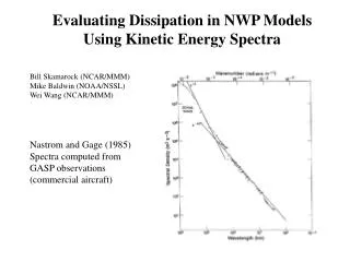
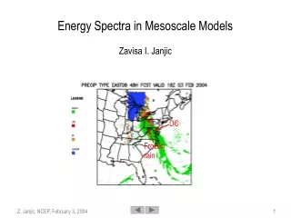
1. Energy Spectra in Mesoscale ModelsZavisa I. Janjic DC Frozen rain 1

2. 108 -3 105 -5/3 104 103 102 101 103 102 ● Nastrom-Gage (1985, JAS) 1D spectrum in upper troposphere and lower stratosphere from commercial aircraft measurements. ● No spectral gap. ● Transition at few hundred kilometers from –3 slope to –5/3 slope. ● 0.01-0.3 m s-1 in the –5/3 range, high up, not to be confused with severe mesoscale phenomena! 2

3. Kreichnan, 1967, Phys. Fluids Lilly, 1989, JAS Tung and Orlando, 2003, JAS 3

4. ● Models with simpler dynamics and coarser resolution can reproduce the –5/3 slope in the statistical sense when averaged over an extended period of time (e.g., Hamilton et al., 1999; Koshyik and Hamilton 2001; Tung and Orlando, 2003). Tung and Orlando, 2003, JAS 4

5. Koshyk and Hamilton, 2001, JAS 5

6. 5th International SRNWP Workshop on Non-Hydrostatic Modelling, Bad Orb, Germany • 20th Conference on WAF/16th Conference on NWP, Seattle, WA • 12.8 Evaluating dissipation in NWP models using kinetic energy spectra • William C. Skamarock, NCAR, Boulder, CO; and M. E. Baldwin and W. Wang • Kinetic energy (KE) spectra derived from observations possess a k**(-3) spectral slope for large scales, characteristic of 2D turbulence, and transition to a shallower k**(-5/3) spectra at the mesoscale (i.e. for length scales of O(10-100) km). We have examined KE spectra computed using mesoscale and experimental cloudscale NWP forecasts from the WRF model, the ETA and NMM models from NCEP, and others.High resolution forecasts from the WRF model match the observational spectra well, including the transition in slope.At the highest resolved wavenumbers the WRF model shows a decaying spectra (steeper spectral slope) compared with observations, indicating energy removal by the model's implicit and explicitdissipation mechanisms.The ETA and NMM models reproduce the observed k**(-3) spectra at low wavenumbers but do not show a transition to the mesoscale k**(-5/3) spectral slope at higher wavenumbers, rather they show slopes generally steeper than k**(-3) - even well before the shorter wavelengths are reached.We will present these spectra and discuss their implications for model formulations and NWP applications. 6

7. ● Currently twoWeather Research and Forecasting (WRF) Model mainstream cores: - NCEP Nonhydrostatic Mesoscale Model (NMM) Janjic, Gerrity and Nickovic, 2001, Monthly Weather ReviewJanjic, 2003, Meteorology and Atmospheric Physics Black, Parallelization, Optimization, WRF standards - NCAR Mass Core (MC) Klemp, Skamarock, Dudhia, 2000, Online Wicker and Skamarock, 2002, Monthly Weather Review Klemp, Skamarock, Fuhrer, 2003, Monthly Weather Review Michalakes, 2002 7

8. ♦♦ The NMM ● Nonhydrostatic design built on NWP experience. ● Basic discretization principles (Janjic, 1977, Beitrage) (also Eta): - Controlled nonlinear energy cascade/Energy and Enstrophy conservation; - Cancellation between contributions of the omega-alpha term and the PGF to KE, consistent transformations between KE and potential energy; - Minimization of sigma coordinate errors. 8

9. NMM Formal 4-th order • ● “Isotropicized” horizontal divergence & advection operators on 9-point Arakawa Jacobian stencil (Janjic, 1984, MWR). ● Interchangable flux/advective form in FD (Janjic 1984; Xue 2001, MWR). 9

10. y x’ h,χ,ψ h,χ,ψ h,χ,ψ h,χ,ψ h,χ,ψ h,χ,ψ h,χ,ψ h,χ,ψ y’ h,χ,ψ h,χ,ψ h,χ,ψ h,χ,ψ h,χ,ψ x • ● For rotational flow and cyclic boundary conditions, the horizontal advection of momentum on E grid conserves (Janjic 1984, MWR): • - Enstrophy as defined on staggred grid C Not “seen” by the E grid, cannot be computed directly from the E grid variables - Rotational kinetic energy as defined on staggered grid C 10

11. - Rotational momentum as defined on the semi-staggered grid E. ● General flow: - Momentum as defined on the semi-staggered grid E - Kinetic energy as defined on the semi-staggered grid E • - Rotational momentum as defined on staggered grid C • - Rotational kinetic energy as defined on the semi-staggered grid E - Total energy - Advection of T conserves first and second moments of T. ● Pressure-sigma hybrid (Arakawa and Lamb, 1977). ● Nonsplit in time. ● A PC version on the B grid, same principles (NMM-B). 11

12. The cold bubble test. Potential temperatures after 300 s, 600 s and 900 s in the right hand part of the integration domain extending from the center to 19200 m, and from the surface to 4600 m. The contour interval is 10 K. Potential temperature after 360 s, 540 s, 720 s and 900 s. The area shown extends 16 km along the x axis, and from 0 m to 13200 m along the z axis. The contour interval is 10K. ● The formulation successfully reproduces classical 2D nonhydrostatic solutions. 12

13. ● Upgraded physical package of the NCEP Eta model (Janjic 1990, 1994, MWR; Chen, Janjic and Mitchell, 1997, BLM; Janjic 2000, JAS; Janjic 2001, NCEP Office Note 437). ● NWP, convective cloud runs, PBL LES, resolutions from 50 km to 100 m. ● Reliable. ● THREE TIMES faster than most established NH models, can be further sped up. ● Little noise, no Rayleigh damping and associated extra computational BC at top. ● Operational at NCEP (small domains, driven by the Eta): - HiRes Windows, Fire Weather, On Call. ● Quasi-Operationally run at several other places. ● Very good performance compared to mature NWP models. 13

14. 14

15. 15

16. ♦♦ The MC ● New nonhydrostatic design. ● Basic discretization principles (Klemp, Skamarock, Dudhia, 2000, draft; Wicker and Skamarock, 2002, MWR; Klemp, Skamarock, Fuhrer, 2003,MWR) - Higher order of formal accuracy with spatial filtering for advection terms (5th order in the horizonatal, 3d order in the vertical, 3d order in time); - “Consistency of metric terms” (pressure advection and pressure gradient force). ● Sigma. ● Process splitting (advection slow, other terms fast). 16

17. ● The formulation successfully reproduces classical 2D nonhydrostatic solutions. ● Mixed physical packages of the Eta, GFS and MM5. ● NWP, convective cloud runs, LES, wide range of resolutions. ● Quasi-operational at NCAR, NCEP, … 17

18. ● Due to the nature of the nonlinear energy cascade, statistics of atmospheric spectra generally are investigated: • - In global scale domains; • - In extended integrations (tens or hundreds of days). • ● What one can reasonably expect in mesoscale runs? • - Initial data deviate from statistics; • - Small domains, no downscale cascade from large scales; • - Short integration time compared to nonlinear cascade time scale; • - Physical or spurious sources of energy other than downscale nonlinear cascade needed to generate and maintain the –5/3 spectra. • ● Possible energy sources: • - Physically justified mesoscale forcing; • - Spurious computational nonlinear cascade; • - Other small-scale computational errors such as errors due to topography, etc. 18

19. Skamarock et al.: “High resolution forecasts from the WRF model match the observational spectra well, including the transition in slope.” Somewhat shallower than –3, but nowhere near –5/3 at higher altitudes (green and red lines). Central US, mountains! 19

20. 20

21. -5/3 -3 21

22. -5/3 -3 22

23. -5/3 -3 23

24. -5/3 -3 24

25. -5/3 -3 25

26. -5/3 -3 26

27. -5/3 -3 Straight lines throughout the spectral range with slopes in between –3 and –5/3. No transition in slope. The spectra are getting shallower with resolution. “High resolution forecasts from the WRF model match the observational spectra well, including the transition in slope.” 27

28. Idealized 3D convection. Kessler warm rain 1 km in the horizontal and 500 m in the vertical. Integrated for four hours. Spectrum of w2 at 3000 m averaged over the last hour. (Takemi and Rotuno, 2003, MWR). No sign of inertial range 28

29. ● The WRF-NMM and the NMM-B well qualified for investigating numerical spectra: - Conservation of rotational energy and enstrophy, more accurate nonlinear energy cascade, - Conservation of total energy provides stable integrations without excessive dissipation (either explicit or built-in finite-difference schemes) that could affect properties of model generated spectra, - Hybrid pressure-sigma vertical coordinate system relatively free of errors associated with representation of mountains in the upper troposphere and in the stratosphere where the sigma coordinate errors are largest, - Explicit formulation of dissipative processes allows precise “dosage” of dissipation. 29

30. 630 km 63 km “The ETA and NMM models reproduce the observed k**(-3) spectra at low wavenumbers but do not show a transition to the mesoscale k**(-5/3) spectral slope at higher wavenumbers, rather they show slopes generally steeper than k**(-3) - even well before the shorter wavelengths are reached.” Central domain, sigma 30

31. ● Are the spectra forced by sigma coordinate errors? ● Are the spectra just projections of the topography spectrum? ● How about over ocean? 31

32. Atlantic, NMM-B, 15 km, 32 levels, hybrid 32

33. Eastern Domain, NMM 8 km, 60 levels, hybrid, “Isabel” 33

34. 630 km 63 km Time average over 36-48 hours of the WRF-NMM spectra (blue diamonds) at 300 hPa in the Eastern Domain. The –3 (pink squares) and –5/3 (yellow triangles) slopes are shown for comparison. Run starting from 18 UTC, 09/17/2003 (Isabel), Eta data, 8 km, 60 levels resolution. No lateral diffusion, weak mass divergence damping. 34

35. Decaying 3D turbulence, Fort Sill storm, 112km by 112km by 16.4km, double periodic, resolution 1km, 32 levels, NMM-B, Kessler warm rain. Spectrum of w2 at 700 hPa averaged between hours 3 and 4 of integration time. 35

36. Decaying 3D turbulence, Fort Sill storm, 112km by 112km by 16.4km, double periodic, resolution 1km, 32 levels, NMM-B, Ferrier microphysics. Spectrum of w2 at 700 hPa. 36

37. Decaying 3D turbulence, Fort Sill storm, 112km by 112km by 16.4km, double periodic, resolution 1km, 32 levels, NMM-B, Ferrier microphysics. Spectrum of w2 at 700 hPa averaged between hours 3 and 4 of integration time. 37

38. Pacific, NMM 8 km, 60 levels, hybrid 38

39. No Physics With Physics The Atlantic case, NMM-B, 15 km, 32 Levels 39

40. -3 -5/3 630 km 63 km ♦♦ SUMMARY ● 40

41. - “High resolution forecasts from the WRF model match the observational spectra well, including the transition in slope.”cannot be substantiated by the available data! - There is no evidence that the MC can reproduce the observed spectra realistically. - The NMM (and by extension presumably the Eta) can reproduce the observed spectra well, including the transition in slope. ● Generally, mesoscale models can reproduce the observed Nastrom and Gage (1985, JAS) spectrum in short range runs well, - Provided there is a sufficiently strong, physical or spurious, energy source at smaller scales, and, - Given enough time. 41

42. ● The model physics and numerical errors can provide the energy needed to spin-up the Nastrom and Gage (1985, JAS) spectrum. ● The mechanisms leading to the development of the Nastrom and Gage (1985, JAS) spectrum in reality and in numerical models may differ. ● The control of the nonlinear energy cascade through dissipation alone does not appear to be sufficient. ● The control of the nonlinear energy cascade through energy and enstrophy conservation appears to be important for reproducing the atmospheric spectrum realistically. ● If model spectrum in short-range integrations is physically justified, the shape of the spectrum could be used for tuning dissipation? 42