
Transverse dynamics
E N D
Presentation Transcript
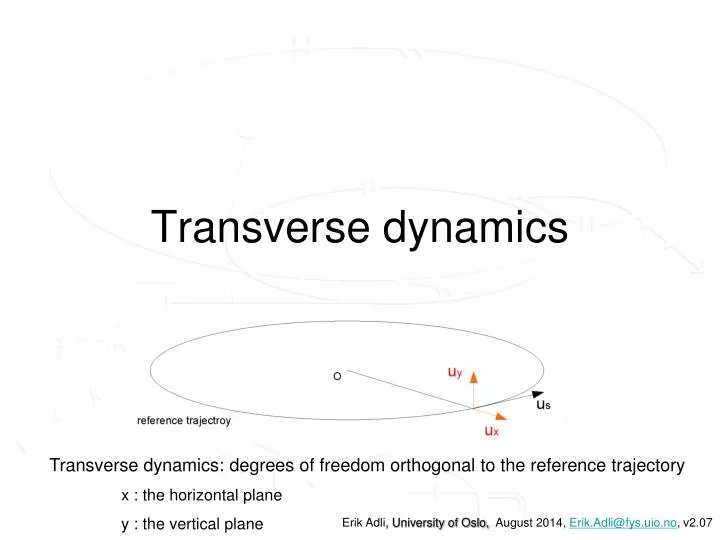
Transverse dynamics Transverse dynamics: degrees of freedom orthogonal to the reference trajectory x : the horizontal plane y : the vertical plane Erik Adli, University of Oslo, August 2014, Erik.Adli@fys.uio.no, v2.07
The reference trajectory • An accelerator is designed around a reference trajectory (often called design orbit in circular accelerators) • This is the trajectory an ideal particle will follow and consist of • a straight line where there is no bending field • arc of circle inside the bending field • We will in the following consider transverse deviations from the reference trajectory, and how to control the magnitude of these deviations
Bending field • Circular accelerators: piecewise circular orbits with a bending radius • straight sections are needed for e.g. particle detectors • in circular arc sections the magnetic field must provide the desired bending radius • The accelerator design specifies a design bending radius, r, for the dipole field bending magnets • In a synchrotron, the bending radius is kept constant during acceleration by synchronization of B and p. B: bending field [T] p: particle momentum [GeV/c] r: design bending radius [m] We define 1/r as the normalized dipole strength :
Focusing field: quadrupole magnets • Reference trajectory: typically through centers of magnets and structures • Desired: a restoring force of the type Fx=-kxin order to keep the particles close to the ideal orbit, in both planes • A linear field in both planes can be derived from the potential V(x,y) = gxy. Four poles with magnet surfaces shaped as hyperbolas. Bx= -gy By = -gx Fx= -qvgx (focusing) Fy = qvgy(defocusing) • Forces are focusing in one plane and defocusing in the orthogonal plane • Opposite focusing/defocusing by rotating the quadrupole by ninety degrees
Normalized magnet strengths • Analogy to dipole strength: normalized quadrupolestrength Quadrupole : g: field gradient [T/m] p: particle momentum [GeV/c] k: design normalized quadrupole strength [m-2] Dipole : B: bending field [T] p: particle momentum [GeV/c] 1/r: design normalized dipole strength [m-1]
Magnetic lenses linear optics • Analogy: magnetic lenses (quadrupoles) linear optics • Focal length fof a quadrupole: where l is the length of the quadrupole • Alternating focusing and defocusing lenses will together give total focusing effect in both planes; “alternating gradient focusing” • f = 1 / kl
The Lattice • An accelerator is composed of bending magnets, focusing magnets and usually also sextupole magnets • The ensemble of magnets in the accelerator constitutes the “accelerator lattice”
Bending field: dipole magnets • Dipole magnets provide uniform field in the desired region • Several design choices, including cos(q)" design that allows opposite and uniform field in both vacuum chambers LHC dipole magnet design
Example: lattice magnets CLIC Test Facility 3
Transverse dynamicsEquations of motion and transfer matrices
Coordinates • Coordinate system: • x, y are small deviations from the reference trajectory • x: deviations in the horizontal plane • y: deviations in the vertical plane • r = r + x • We will outline the steps needed to develop the equations of motion in terms of deviations from the reference trajectory. For full derivation, see Wille (2000).
Linear equations of motion I • Equations of motion in a uniform magnetic field : • In accelerators we use x(s) instead of x(t), and we denotedx/ds = x’(s). • Furthermore, using vx << v, we write yielding the equation of motion as function of the accelerator coordinate s : B: dipole field g: quadrupole field gradient ( assuming g >> 1 ) ( Corresponding equations for y )
Linear equations of motion II • Further approximations, and dropping higher order terms : • We introduce the normalized magnet strengths: • By substituting the above we obtain the linearized trajectory equations: • k: normalized quadrupole strength • 1/r:normalized dipole strength • p0 is the reference momentum, Dp is deviation from ideal momentum
Hill’s equation • Magnet strength terms are dependent on the position along the reference trajectory, s. We can then write eq. of motion as a Hill's equation: • 1/r2(s) – k(s) K(s) • We assume first Dp=0, yielding the homogenous Hill’s equation: • We write equations for x, analogous for y • For a given magnet lattice: we take a piece-wise approach to solution: • For K(s) = const>0, solutions is: • K(s)=const <0: replace with hyperbolic functions • It is helpful to put the coefficients into a matrix, the transfer matrix :
M: drift space • The element with the simplest transfer matrix M: drift space between magnets (no field), with length l : • Written out this gives: • This simply says that in a drift space x’ is unchanged, and x drifts
Quadrupole transfer matrix k [m-2] • Full solution : • Thin lens approximation : • Real quadrupolemay be modeled as a infinitely thin lens that focuses or defocuses, plus the drift space to represent the length of the quadrupole • valid if focal length f=1/kl >> l • Written out multiplication: • -1/f is a focusing term • A defocusing quadrupole in x (rotated 90): -f f l [m]
Dipole transfer matrix • Bending magnets introduce focusing terms as well. • The solution of Hill’s equation provides the focusing terms for a idealized sector dipole : • The more common type of dipole found in accelerators is a rectangular dipole, which does not provide the focusing term.
Hill’s equation:solutions for an accelerator • The transverse optics of an accelerator can be modelled as composed of elements where K(s) = constant inside the element • We solve Hill’s equation by applying the transfer matrix M, from the start to the end of each element • Inside dipoles: K(s) = 1/r2 • Inside quadrupoles: K(s) = +/-k • Where there is no field: K(s) = 0 • One can find the effect on a particle travelling through the whole, or part, of the lattice by multiplying the M matrices for the various components:
Quadrupole FODO doublet • A FODO quadrupole doublet consist of a focusing quadrupole followed by a drift, a defocusing quadrupole and a drift • Using the thin lens approximation we can calculate the total matrix : • FODO is focusing in both the horizontal and the vertical planes (since changing plane equals f = -f )
Stability of a FODO structure • A FODO lattice yields focusing in both planes, however too short focal length will give overfocusing, and an unstable trajectory: • We may calculate rigorously the stability criterion of a periodic lattice using Courant-Snyder analysis introduced in the next section Liming case, L = 4 f
Transverse dynamicsCourant-Snyder framework Previous section: a straight-forward mathematical framework for computing single particle motion The next slides : analyze the transverse motion in an accelerators using standard accelerator terminology, allowing for analysis of a beam of particles
Particle motion: Hill's equation • We have calculated particle motion for a single particle by solving Hill’s equation piece-wise and multiplying transfer matrices M(s). We now seek a general solution of the the equation : • Reminder: solution of Hill’s equation with K(s) =K harmonic oscillator
Reformulation of Hill's equation: beta function We define function varying along the lattice in the solution to the Hill’s equation; the beta function, b(s). The solution is thus a quasi-harmonic oscillator, with amplitude and phase-advance dependent on s. The complete solution is given by solving the betatron equation (left).
Transverse phase-space • The particle phase-spacein the horizontal plane is spanned by xand x‘: • By eliminating the phase, f, we get equation for an ellipsewith area pe : where we have defined : a(s) -(1/2)b'(s), g(s) (1+ a2(s))/ b(s), b(s), a(s), g(s): Twiss parameters (in the USA: called Courant-Snyder parameters) e : single particle emittance For a given single particleemittance, e, thephase-spaceellipse area is an invariant (withrespect to thescoordinate).
The phase-space ellipse Envelope of particle motion : Particles with different phase and equal emittance.
Evolution of the phase-space ellipse • Particles populate trajectories on ellipses with the shape determined by the Twiss parameters, b, a, g. • The Twiss parameters evolve according to the solution of Hill’s equation, i.e. they depend on the position along the lattice, s • As they evolve, the area of the ellipse, pe, remains constant From A. Chao
Single particle propagation In the Courant-Snyder framework, which information do we need to describe the propagation of a single particle? 1) We need the Twiss parameters. These are given as solutions of the betatron equation. How they propagate depends only on the lattice specification, K(s) : 2) In addition, the particle initial state must be specified, by the initial single particle emittance, e, and its initial phase f0. This is hardly a simplification of the single particle motion, however, we shall now relate the Twiss parameters and the description of the entire beam.
Twiss parameters: initial conditions For a non-circular lattice, the solution of Hill’s equation, the Twiss parameters, depends on the initial Twiss parameters(the initial beam), b(0) and a(0)=-1/2b’(0). Usually the lattice has design Twiss parameters, and one aims to match the incoming beam to the lattice design. Example to the right: evolution of Twiss parameters where the initial magnets are adjusted to match the beam into a periodic focusing lattice of FODO-type. Example from the CLIC Test Facility at CERN F D
Betatron oscillations and phase advance Solution of Hill’s equation : Example solution in a periodic lattice : • A particle will undergo betatron oscillations around the reference trajectory. The lattice parameter b(s) defines the envelope for the particle motion • f(s) isthe particle phase-advance from point s0 to point s in a lattice • In a FODO structure the beta function is at maximum in the middle of the F quadrupole and at minimum in the middle of the D quadrupole • In the figure : about 5 FODO cells for a full oscillation, yielding a phase-advance per FODO cell offcell 70º.
Evolution of beams The importance of this is that we can describe the transport of the 2nd order moments of the beam in the same way as we describe the transformation of the Twiss parameters along the lattice. For Gaussian beams and linear optics, this means that the Twiss parameters uniquely defines the beam shape along the lattice.
Relation b(s) and M(s) • We calculated earlier the evolution of single particles along an accelerator lattice using the transfer matrices: x1= M10x0 • We can calculate the evolution of the beta function using transfer matrices as well. We define a matrix with the Twiss parameters : • The solution of Hill's gives: xTB-1 (s)x= const. • Substituting x1 = Mx0gives :
Emittance preservation • We have shown that the rmsemittance is a preserved quantity for Gaussian beams, in drift and with linear magnetic lenses • More generally the phase-space area, emittance, is preserved if only conservative forces do work on the particles (Liouville’s theorem) • Particle acceleration by an RF-field is not conservative, the emittance will shrink if the beam is accelerated : • The emittance will shrink proportional to the beam energy increase, given by bg,. We define a normalized emittance, conserved under acceleration : NB: b g on this slide is the normalized velocity and the Lorentz factor respectively. They are not related to the Twiss parameters. eN,rms = gberms Independent quantities in each plane, x, y.
Periodic lattices • Consider a periodicaccelerator lattice, withMss+L(s) from point s to point s+L. For example, one full turn of a circular accelerator may be the period. • The Twiss parameters must obey the following condition : • The parameters are in this case uniquely defined byMss+L(s) : Circular accelerators: periodic lattice by default. Existence of periodic solutions follows by Floquet Theory.
Twiss parameters: period lattice Using the solution of Hill’s equation we may re-write the transfer matrix between two locations in an accelerator in terms of Twiss parameters as : For a periodic lattice, with period L, this reduces to : where F = y(s2) – y(s1)is the phase-advance from s1 to s2. The lattice Twiss parameters may then be calculated from the periodic transfer matrix :
Example: thin-lens FODO f L Example from A. Chao
Stability of a lattice • Absolute requirement: the lattice structure of an accelerator must be stable: motion must be bounded • Let M(s) be the matrix for one periodic cell, M(s)N is the matrix for the whole accelerator,. M(s)nN corresponds to n turns in the accelerator • Stability requires that the elements of M(s)nN remain bounded as n • Applying this general criterion on the FODO cell gives the condition : Liming case, L = 4 f
Particle motion in a periodic lattice, tune Reminder: even if beta function is be periodic, the particle motion itself is in general notperiodic; after one revolution the initial phase f0 is altered, since the particle has advanced by a certain phase,fturn.Phase advance per turn may be given as the number of periodic cells, and the phase-advance per cell, fturn = Ncellfcell . • We define the tune, Q, as the number of betatron oscillations per turn : • Q = Ncellfcell/ 2p (From M. Sands)
Tune diagram • In order to avoid driving resonant instabilities in a circular accelerator, the fractional part of the tune, Q, must not be mQx + nQy = N, where m,n,Nmay be 0,1,2,3….(up to a number depending on the performance requirements). • These instabilities originate from imperfections of real magnets; beam undergoes small kicks, which if they add up coherently may blow up beam size. Integer and N-integer tunes must be avoided
Evolution of a beam Rmsbeam size: Beam quality Evolves with lattice
Summary: Transverse parameters • Betatronoscillations: particle oscillations in the transverse planes, due to the focusing, for example alternating gradient focusing • b(s):beta function square of envelope of the particle motion • in periodic accelerators: defined uniquely by the lattice • e : emittance, measurement of beam quality; conserved under conservative forces • Q = Ncellfcell / 2p : accelerator tune • Integer and half-integer tunes etc. will lead to instabilities and must be avoided • An alternative expression for luminosity:
Acknowledgements • Part of the material presented here is based on Alex Chao’s USPAS lecture notes and Volker Ziemann’s lecture notes.