Probability and Statistics Refresher: Fundamentals and Applications

1. A Refresher on Probability and Statistics Appendix C Last revision August 26, 2003 Appendix C – A Refresher on Probability and Statistics

2. What We’ll Do ... • Ground-up review of probability and statistics necessary to do and understand simulation • Assume familiarity with • Algebraic manipulations • Summation notation • Some calculus ideas (especially integrals) • Outline • Probability – basic ideas, terminology • Random variables, joint distributions • Sampling • Statistical inference – point estimation, confidence intervals, hypothesis testing Appendix C – A Refresher on Probability and Statistics

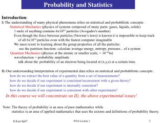
3. Probability Basics • Experiment – activity with uncertain outcome • Flip coins, throw dice, pick cards, draw balls from urn, … • Drive to work tomorrow – Time? Accident? • Operate a (real) call center – Number of calls? Average customer hold time? Number of customers getting busy signal? • Simulate a call center – same questions as above • Sample space – complete list of all possible individual outcomes of an experiment • Could be easy or hard to characterize • May not be necessary to characterize Appendix C – A Refresher on Probability and Statistics

4. Probability Basics (cont’d.) • Event – a subset of the sample space • Describe by either listing outcomes, “physical” description, or mathematical description • Usually denote by E, F, E1, E2, etc. • Union, intersection, complementation operations • Probability of an event is the relative likelihood that it will occur when you do the experiment • A real number between 0 and 1 (inclusively) • Denote by P(E), P(EF), etc. • Interpretation – proportion of time the event occurs in many independent repetitions (replications) of the experiment • May or may not be able to derive a probability Appendix C – A Refresher on Probability and Statistics

5. Probability Basics (cont’d.) • Some properties of probabilities If S is the sample space, then P(S) = 1 Can have event ES with P(E) = 1 If Ø is the empty event (empty set), then P(Ø) = 0 Can have event E Ø with P(E) = 0 If EC is the complement of E, then P(EC) = 1 – P(E) P(EF) = P(E) + P(F) – P(EF) If E and F are mutually exclusive (i.e., EF = Ø), then P(EF) = P(E) + P(F) If E is a subset of F (i.e., the occurrence of E implies the occurrence of F), then P(E) P(F) If o1, o2, … are the individual outcomes in the sample space, then Appendix C – A Refresher on Probability and Statistics

6. Probability Basics (cont’d.) • Conditional probability • Knowing that an event F occurred might affect the probability that another event E also occurred • Reduce the effective sample space from S to F, then measure “size” of E relative to its overlap (if any) in F, rather than relative to S • Definition (assuming P(F)  0): • E and F are independent if P(EF) = P(E) P(F) • Implies P(E|F) = P(E) and P(F|E) = P(F), i.e., knowing that one event occurs tells you nothing about the other • If E and F are mutually exclusive, are they independent? Appendix C – A Refresher on Probability and Statistics

7. Random Variables • One way of quantifying, simplifying events and probabilities • A random variable (RV) is a number whose value is determined by the outcome of an experiment • Technically, a function or mapping from the sample space to the real numbers, but can usually define and work with a RV without going all the way back to the sample space • Think: RV is a number whose value we don’t know for sure but we’ll usually know something about what it can be or is likely to be • Usually denoted as capital letters: X, Y, W1, W2, etc. • Probabilistic behavior described by distribution function Appendix C – A Refresher on Probability and Statistics

8. Discrete vs. Continuous RVs • Two basic “flavors” of RVs, used to represent or model different things • Discrete – can take on only certain separated values • Number of possible values could be finite or infinite • Continuous – can take on any real value in some range • Number of possible values is always infinite • Range could be bounded on both sides, just one side, or neither Appendix C – A Refresher on Probability and Statistics

9. Discrete Distributions • Let X be a discrete RV with possible values (range) x1, x2, … (finite or infinite list) • Probability mass function (PMF) p(xi) = P(X = xi) for i = 1, 2, ... • The statement “X = xi” is an event that may or may not happen, so it has a probability of happening, as measured by the PMF • Can express PMF as numerical list, table, graph, or formula • Since X must be equal to somexi, and since the xi’s are all distinct, Appendix C – A Refresher on Probability and Statistics

10. Discrete Distributions (cont’d.) • Cumulative distribution function (CDF) – probability that the RV will be  a fixed value x: • Properties of discrete CDFs 0 F(x)  1 for all x As x –, F(x)  0 As x +, F(x)  1 F(x) is nondecreasing in x F(x) is a step function continuous from the right with jumps at the xi’s of height equal to the PMF at that xi These four properties are also true of continuous CDFs Appendix C – A Refresher on Probability and Statistics

11. Discrete Distributions (cont’d.) • Computing probabilities about a discrete RV – usually use the PMF • Add up p(xi) for those xi’s satisfying the condition for the event • With discrete RVs, must be careful about weak vs. strong inequalities – endpoints matter! Appendix C – A Refresher on Probability and Statistics

12. Discrete Expected Values • Data set has a “center” – the average (mean) • RVs have a “center” – expected value • Also called the mean or expectation of the RV X • Other common notation: m, mX • Weighted average of the possible values xi, with weights being their probability (relative likelihood) of occurring • What expectation is not: The value of X you “expect” to get E(X) might not even be among the possible values x1, x2, … • What expectation is: Repeat “the experiment” many times, observe many X1, X2, …, Xn E(X) is what converges to (in a certain sense) as n Appendix C – A Refresher on Probability and Statistics

13. Discrete Variances andStandard Deviations • Data set has measures of “dispersion” – • Sample variance • Sample standard deviation • RVs have corresponding measures • Other common notation: • Weighted average of squared deviations of the possible values xi from the mean • Standard deviation of X is • Interpretation analogous to that for E(X) Appendix C – A Refresher on Probability and Statistics

14. Continuous Distributions • Now let X be a continuous RV • Possibly limited to a range bounded on left or right or both • No matter how small the range, the number of possible values for X is always (uncountably) infinite • Not sensible to ask about P(X = x) even if x is in the possible range • Technically, P(X = x) is always 0 • Instead, describe behavior of X in terms of its falling between two values Appendix C – A Refresher on Probability and Statistics

15. Continuous Distributions (cont’d.) • Probability density function (PDF) is a function f(x) with the following three properties: f(x)  0 for all real values x The total area under f(x) is 1: For any fixed a and b with ab, the probability that X will fall between a and b is the area under f(x) between a and b: • Fun facts about PDFs • Observed X’s are denser in regions where f(x) is high • The height of a density, f(x), is not the probability of anything – it can even be > 1 • With continuous RVs, you can be sloppy with weak vs. strong inequalities and endpoints Appendix C – A Refresher on Probability and Statistics

16. Continuous Distributions (cont’d.) • Cumulative distribution function (CDF) - probability that the RV will be  a fixed value x: • Properties of continuous CDFs 0 F(x)  1 for all x As x –, F(x)  0 As x +, F(x)  1 F(x) is nondecreasing in x F(x) is a continuous function with slope equal to the PDF: f(x) = F'(x) F(x) may or may not have a closed-form formula These four properties are also true of discrete CDFs Appendix C – A Refresher on Probability and Statistics

17. Continuous Expected Values, Variances, and Standard Deviations • Expectation or mean of X is • Roughly, a weighted “continuous” average of possible values for X • Same interpretation as in discrete case: average of a large number (infinite) of observations on the RV X • Variance of X is • Standard deviation of X is Appendix C – A Refresher on Probability and Statistics

18. Joint Distributions • So far: Looked at only one RV at a time • But they can come up in pairs, triples, …, tuples, forming jointly distributed RVs or random vectors • Input: (T, P, S) = (type of part, priority, service time) • Output: {W1, W2, W3, …} = output process of times in system of exiting parts • One central issue is whether the individual RVs are independent of each other or related • Will take the special case of a pair of RVs (X1, X2) • Extends naturally (but messily) to higher dimensions Appendix C – A Refresher on Probability and Statistics

19. Joint Distributions (cont’d.) • Joint CDF of (X1, X2) is a function of two variables • Same definition for discrete and continuous • If both RVs are discrete, define the joint PMF • If both RVs are continuous, define the joint PDFf(x1, x2) as a nonnegative function with total volume below it equal to 1, and • Joint CDF (or PMF or PDF) contains a lot of information – usually won’t have in practice Replace “and” with “,” Appendix C – A Refresher on Probability and Statistics

20. Marginal Distributions • What is the distribution of X1 alone? Of X2 alone? • Jointly discrete • Marginal PMF of X1 is • Marginal CDF of X1 is • Jointly continuous • Marginal PDF of X1 is • Marginal CDF of X1 is • Everything above is symmetric for X2 instead of X1 • Knowledge of joint  knowledge of marginals – but not vice versa (unless X1 and X2 are independent) Appendix C – A Refresher on Probability and Statistics

21. Covariance Between RVs • Measures linear relation between X1 and X2 • Covariance between X1 and X2 is • If large (resp. small) X1 tends to go with large (resp. small) X2, then covariance > 0 • If large (resp. small) X1 tends to go with small (resp. large) X2, then covariance < 0 • If there is no tendency for X1 and X2 to occur jointly in agreement or disagreement over being big or small, then Cov = 0 • Interpreting value of covariance – difficult since it depends on units of measurement Appendix C – A Refresher on Probability and Statistics

22. Correlation Between RVs • Correlation (coefficient) between X1 and X2 is • Has same sign as covariance • Always between –1 and +1 • Numerical value does not depend on units of measurement • Dimensionless – universal interpretation Appendix C – A Refresher on Probability and Statistics

23. Independent RVs • X1 and X2 are independent if their joint CDF factors into the product of their marginal CDFs: • Equivalent to use PMF or PDF instead of CDF • Properties of independent RVs: • They have nothing (linearly) to do with each other • Independence  uncorrelated • But not vice versa, unless the RVs have a joint normal distribution • Important in probability – factorization simplifies greatly • Tempting just to assume it whether justified or not • Independence in simulation • Input: Usually assume separate inputs are indep. – valid? • Output: Standard statistics assumes indep. – valid?!? Appendix C – A Refresher on Probability and Statistics

24. Sampling • Statistical analysis – estimate or infer something about a population or process based on only a sample from it • Think of a RV with a distribution governing the population • Random sample is a set of independent and identically distributed (IID) observations X1, X2, …, Xn on this RV • In simulation, sampling is making some runs of the model and collecting the output data • Don’t know parameters of population (or distribution) and want to estimate them or infer something about them based on the sample Appendix C – A Refresher on Probability and Statistics

25. Population parameter Population mean m = E(X) Population variance s2 Population proportion Parameter – need to know whole population Fixed (but unknown) Sample estimate Sample mean Sample variance Sample proportion Sample statistic – can be computed from a sample Varies from one sample to another – is a RV itself, and has a distribution, called the sampling distribution Sampling (cont’d.) Appendix C – A Refresher on Probability and Statistics

26. Sampling Distributions • Have a statistic, like sample mean or sample variance • Its value will vary from one sample to the next • Some sampling-distribution results • Sample mean If Regardless of distribution of X, • Sample variance s2 E(s2) = s2 • Sample proportion E( ) = p Appendix C – A Refresher on Probability and Statistics

27. Point Estimation • A sample statistic that estimates (in some sense) a population parameter • Properties • Unbiased: E(estimate) = parameter • Efficient: Var(estimate) is lowest among competing point estimators • Consistent: Var(estimate) decreases (usually to 0) as the sample size increases Appendix C – A Refresher on Probability and Statistics

28. Confidence Intervals • A point estimator is just a single number, with some uncertainty or variability associated with it • Confidence interval quantifies the likely imprecision in a point estimator • An interval that contains (covers) the unknown population parameter with specified (high) probability 1 – a • Called a 100 (1 – a)% confidence interval for the parameter • Confidence interval for the population mean m: • CIs for some other parameters – in text tn-1,1-a/2 is point below which is area 1 – a/2 in Student’s t distribution with n – 1 degrees of freedom Appendix C – A Refresher on Probability and Statistics

29. Confidence Intervals in Simulation • Run simulations, get results • View each replication of the simulation as a data point • Random input  random output • Form a confidence interval • Brackets (with probability 1 – a) the “true” expected output (what you’d get by averaging an infinite number of replications) Appendix C – A Refresher on Probability and Statistics

30. Hypothesis Tests • Test some assertion about the population or its parameters • Can never determine truth or falsity for sure – only get evidence that points one way or another • Null hypothesis (H0) – what is to be tested • Alternate hypothesis (H1 or HA) – denial of H0 H0: m = 6 vs. H1: m 6 H0: s < 10 vs. H1: s 10 H0: m1 = m2 vs. H1: m1m2 • Develop a decision rule to decide on H0 or H1 based on sample data Appendix C – A Refresher on Probability and Statistics

31. Errors in Hypothesis Testing Appendix C – A Refresher on Probability and Statistics

32. p-Values for Hypothesis Tests • Traditional method is “Accept” or Reject H0 • Alternate method – compute p-value of the test • p-value = probability of getting a test result more in favor of H1 than what you got from your sample • Small p (like < 0.01) is convincing evidence against H0 • Large p (like > 0.20) indicates lack of evidence against H0 • Connection to traditional method • If p < a, reject H0 • If pa, do not reject H0 • p-value quantifies confidence about the decision Appendix C – A Refresher on Probability and Statistics

33. Hypothesis Testing in Simulation • Input side • Specify input distributions to drive the simulation • Collect real-world data on corresponding processes • “Fit” a probability distribution to the observed real-world data • Test H0: the data are well represented by the fitted distribution • Output side • Have two or more “competing” designs modeled • Test H0: all designs perform the same on output, or test H0: one design is better than another • Selection of a “best” model scenario Appendix C – A Refresher on Probability and Statistics