Illustrating Smooth Surfaces
380 likes | 429 Views
Illustrating Smooth Surfaces. Aaron Hertzmann Denis Zorin New York University Presented by Mark Blackburn, Fall 2005. Organization. Motivation Contributions Related Work Process Results Conclusion & Future Work. Motivation.

Illustrating Smooth Surfaces
E N D
Presentation Transcript
Illustrating Smooth Surfaces Aaron Hertzmann Denis Zorin New York University Presented by Mark Blackburn, Fall 2005
Organization • Motivation • Contributions • Related Work • Process • Results • Conclusion & Future Work
Motivation • Silhouette drawing often insufficient for drawing objects that are complex or free-form. • A smooth object may have no visible silhouette lines except the outer silhouette and all the information inside the silhouette may be lost (cf. Figure 1) • Adding lines can convey the complexity of the shape • Line drawing often conveys info better than a photograph. Figure 1
Contributions Three Algorithms • Silhouette detection • Cusp detection and segmentation • Computing smooth direction fields
Related Work • Image-space vs. Object-space NPR • Silhouette detection • Randomized algorithm (fast, but does not guarantee to find all surfaces) • Gauss map (only works in orthographic projection) • This paper presents an algorithm that is fast, deterministic, and is applicable to orthographic as well as perspective projections
Related Work • Computing smooth direction fields: • Parametric lines on NURBS • Parameterization does not exist for many types of surfaces • Principal Curvature Hatching • Can’t be reliably or uniquely computed at many surface points • Intersections of the surfaces with planes • Requires segmentation of the surface into parts where different groups of planes are used • Plane orientations computed using skeletons relate only indirectly to the local surface properties
Process Overview Input:Polygonal Mesh (Stage 1) Hatch Direction Field:Defines a view-independent cross-field that can be used later to generate hatches (Stage 2) Silhouette Curve computation:Computes all curves, creases, cusps, and determines the visibility and segmentation of all silhouette curves (Stage 3) Hatch Generation:Divides surface into four levels of brightness (highlights, midtones, shadows, and undercuts) and generates hatches for each area of the surface Output:Illustrated Image
Stage 1:Hatch Fields Determine hatch direction fields for entire surface • Choice of direction field algorithm guided by these three observations: • Surface geometry is rendered best by principal curvature directions on cylindrical surfaces • Isoparametric lines work well as curvature directions when a parameterization exists and is close to isometric • Artists tend to use relatively straight hatch lines, even when the surface has wrinkles. Smaller details are conveyed by varying the density and the number of hatch directions.
Stage 1:Hatch Fields Simple requirements for hatching fields • In areas where the surface is close to parabolic, the field should be close to principal curvature directions • On the whole surface, the integral curves of the fields should be close to geodesic • If the surface has small details, the field should be generated using a smoothed version of the surface
Stage 1:Hatch Fields Four steps to determine hatch direction field • (Optional) Create a smoothed copy of the original mesh (User specified) • Identify areas of surface which are sufficiently close to parabolic • Initialize field over the surface by computing principal curvature directions • Fix the quasi-parabolic areas and *optimize* the rest of the vertices.
Stage 2: Silhouette Curves Definition • A silhouette drawing includes only the images of the most visually important curves on the surface: boundaries, creases, silhouette lines, and self-intersection lines
Stage 2: Silhouette Curves • Problem: There are significant differences between the silhouettes of smooth surfaces and their approximating polygonal meshes • For polygonal meshes, complex cusps, where several silhouette chains meet, are stable (do not disappear when the viewpoint is perturbed) • For smooth surfaces, the only type of stable singularity is a simple cusp.
Stage 2: Silhouette Curves Examples
Stage 2: Silhouette Curves • Silhouette detection: • First, we find the silhouette set • Silhouette set is the set of points p of the surface such that: g(p) = (n(p) • (p-c)) = 0 • We compute an approximation to g(p) by computing the true surface normal and g(p) for each vertex and then linearly interpolating the values of the function. • The zero set of this function will consist of line segments inside each triangle of the polygonal approximation.
Stage 2: Silhouette Curves • Cusp Detection: cusps are the points where the tangent plane is parallel to the view direction • Cusp function: C(p) = K1(v • w1)2 +K2(v • w2)2
Stage 2: Silhouette Curves • Cusps are contained in the intersection set of the two families of curves: the zero set of g(p) and zero set of C(p). Cusps = { g(p) = 0 C(p) = 0}
Stage 2: Silhouette Curves • Optimization: Eliminate need to traverse entire mesh. • Duality Map: Map surface M M’ • M’ can be obtained by mapping each point of M to a homogeneous point N = [n1, n2, n3, - (p • n)] where n = [n1, n2, n3,0] is the unit normal at p.
Stage 2: Silhouette Curves • If we let C = [c1, c2, c3, c4] be our viewpoint in the homogeneous form, then the silhouette of the surface consists of all points p for which C is in the tangent plane at that point. • Finding the surface is reduced to the problem of intersecting a plane with a surface for which many space-partition-based acceleration techniques are available.
Stage 2: Silhouette Curves Dual Map
Stage 2: Silhouette Curves Planar Projections
Stage 2: Silhouette Curves Fast Silhouette Detection • For each vertex p, with normal n, we compute the dual position N = [n1, n2, n3, - (p • n)] • Normalize each dual position N using l∞-norm • Each triangle of dual mesh is assigned to a list for every 3D space in which it has a vertex • An octree is constructed for each 3D face and the triangles assigned to this face are placed in the octree
Stage 3: Hatch Generation • Surface is separated into four levels of hatching:
Stage 3: Hatch Generation • Basic rules: • If there is an undercut, on the other side of the silhouette from a fold, a thin area along the silhouette on the fold side is not hatched • Undercuts are densely hatched • Hatches are approximately straight • Optionally, hatch thickness within each density level can be made inversely proportional to lighting
Stage 3: Hatch Generation • Hatching has several user tunable parameters: • Basic hatch density • Hatch density for undercuts • Threshold for highlights • Threshold for transition from single to cross hatch • Max hatch length • Max hatch deviation from initial direction • Varying these parameters has considerable effect both on the appearance of the images and the time required by the algorithm
Stage 3: Hatch Generation • Hatch placement process: • Identify Mach bands and undercuts • Cover single and cross-hatch regions with cross hatches, and add extra hatches to undercut regions • Remove cross-hatches in the single hatch regions, leaving only one direction of hatches
Stage 3: Hatch Generation • Identifying Mach Bands • Step along each silhouette and boundary curve • Use ray test near each curve point to determine if fold overlaps another surface • Undercuts and Mach Bands are indicated in a 2D grid by marking every grid cell within a small distance of the fold on the near side of the surface as a Mach Band
Stage 3: Hatch Generation • Cross-Hatching: • Create evenly spaced cross hatches on a surface • Creates a queue of surface curves • Dequeue each curve and seed it with cross-hatches by tracing direction of field • Hatches are also seeded parallel to other hatches (distance determined by tunable param) • Hatches are seeded perpendicular to all curves • A hatch continues along a curve until it terminates in a critical curve, deviates from direction more than ‘Max’ param, or until it comes near a parallel hatch
Stage 3: Hatch Generation • Hatch Reduction • Once we have cross-hatched all hatch regions, we remove hatches from the single hatch regions until they contain no cross-hatches • Algorithm implicitly segments the visible single-hatch regions into locally consistent single hatching fields • Use a breadth-first traversal of hatches.
Results Mathematical surfaces
Conclusion • Advantages: • Beautiful images that mirror pen-and-ink illustrations • Technique can be used in orthographic or perspective projections • User tunable • Disadvantages: • Performance varies significantly based on parameters and model (seconds to minutes) • Parameters have to be chosen carefully which may take several iterations to get desired result
Future Work • Improvements should be made to the silhouette visibility algorithm • Performance speedups are possible • Reduce the number of user parameters • Hatch reduction algorithm could be more robust
References • Aaron Hertzmann and Denis Zorin, "Illustrating Smooth Surfaces," Siggraph 00, pp. 517 - 526.