Mean-shift and its application for object tracking
310 likes | 498 Views
Mean-shift and its application for object tracking. Dorin Comaniciu, Visvanathan Ramesh and Peter Meer “Kernel-Based Object Tracking”, IEEE Transactions on Pattern Analysis and Machine Intelligence, vol.25, No 5, May 2003

Mean-shift and its application for object tracking
E N D
Presentation Transcript
Mean-shift and its application for object tracking Dorin Comaniciu, Visvanathan Ramesh and Peter Meer “Kernel-Based Object Tracking”, IEEE Transactions on Pattern Analysis and Machine Intelligence, vol.25, No 5, May 2003 Dorin Comaniciu and Peter Meer, “Mean shift: a robust approach toward feature space analysis”, IEEE Transactions on Pattern Analysis and Machine Intelligence, vol.25, no 5, May 2002 Dorin Comaniciu and Peter Meer, “Mean shift analysis and applications", The Proceedings of the Seventh IEEE International Conference on Computer Vision, vol.2, pp.1197-1203, September 1999 Andy {andrey.korea@gmail.com}
What is mean-shift? Data A tool for: finding modes in a set of data samples, manifesting an underlying probability density function (PDF) in RN Non-parametric Density Estimation Discrete PDF Representation Non-parametric Density GRADIENT Estimation (Mean Shift) PDF Analysis
Intuitive description Objective : Find the densest region Region of interest Center of mass Mean Shift vector
Intuitive description Objective : Find the densest region Region of interest Center of mass Mean Shift vector
Intuitive description Objective : Find the densest region Region of interest Center of mass Mean Shift vector
Intuitive description Objective : Find the densest region Region of interest Center of mass Mean Shift vector
Intuitive description Objective : Find the densest region Region of interest Center of mass Mean Shift vector
Intuitive description Objective : Find the densest region Region of interest Center of mass Mean Shift vector
Intuitive description Objective : Find the densest region Region of interest Center of mass
Modality analysis Tessellate the space with windows Run the procedure in parallel
Modality analysis The blue data points were traversed by the windows towards the mode
Modality analysis Window tracks signify the steepest ascent directions
Data clustering example Simple Modal Structures Complex Modal Structures
Data clustering example Feature space: L*u*v representation Initial window centers Modes found Modes after pruning Final clusters
General framework: target representation Choose a reference model in the current frame Choose a feature space Represent the model in the chosen feature space … … Current frame
General framework: target localization Search in the model’s neighborhood in next frame Find best candidate by maximizing a similarity func. Model Candidate … … Current frame Start from the position of the model in the current frame Repeat the same process in the next pair of frames
Target representation Choose a reference target model Choose a feature space Represent the model by its PDF in the feature space Quantized Color Space
PDF representation SimilarityFunction: Target Model (centered at 0) Target Candidate (centered at y)
Smoothness of the similarity function Similarity Function: Target is represented by color info only Spatial info is lost Large similarity variations for adjacent locations Problem: f is not smooth Gradient-based optimizations are not robust Mask the target with an isotropic kernel in the spatial domain f(y) becomes smooth in y Solution:
PDF with spatial weighting candidate model y 0 • A differentiable, isotropic, convex, monotonically decreasing kernel • Peripheral pixels are affected by occlusion and background interference The color bin index (1..m) of pixel x Probability of feature u in model Probability of feature u in candidate Normalization factor Normalization factor Pixel weight Pixel weight Target pixel locations
Similarity function The Bhattacharyya Coefficient 1 1 Target model: Target candidate: Similarity function:
Target localization algorithm Search in the model’s neighborhood in next frame Find best candidate by maximizing a similarity func. Start from the position of the model in the current frame
Approximating similarity function Linear approx. (around y0) Model location: Candidate location: Independent of y Density estimation (as a function of y)
Computing gradient of similarity function • Simple Mean Shift procedure: • Compute mean shift vector • Translate the Kernel window by m(x)
Kernels and kernel profiles k – kernel profile K– kernel • Epanechnikov Kernel • Uniform Kernel • Normal Kernel
Epanechnikov kernel Uniform kernel: A special class of radially symmetric kernels: Epanechnikov kernel:
Tracking with mean-shift 1. Initialize the location of the target in the current frame (y0)with location of model on previous frame, compute candidate target model p(y0) and evaluate 2. Compute weights 3. Find the next location of the target candidate according to 4. Compute candidate model at new position p(y1) 5. If ||y0-y1||<ε Stop. Else – set y0 = y1 and go to step 2.
Conclusions • Advantages : • Application independent tool • Suitable for real data analysis • Does not assume any prior shape (e.g. elliptical) on data clusters • Can handle arbitrary feature spaces • Only ONE parameter to choose • h (window size) has a physical meaning, unlike K-Means • Disadvantages: • The window size (bandwidth selection) is not trivial • Inappropriate window size can cause modes to be merged, or generate additional “shallow” modes Use adaptive window size