Download
1 / 44
440 likes | 569 Views
Truthful Randomized Mechanisms for Combinatorial Auctions. Speaker: Shahar Dobzinski Joint work with Noam Nisan and Michael Schapira. Combinatorial Auctions. A set of indivisible different items is for sale Items might be: Complements : v(TV) + v(VCR) < v(TV+VCR)

E N D
Truthful Randomized Mechanisms for Combinatorial Auctions Speaker: Shahar Dobzinski Joint work with Noam Nisan and Michael Schapira
Combinatorial Auctions • A set of indivisible different items is for sale • Items might be: • Complements: v(TV) + v(VCR) < v(TV+VCR) • Substitutes:v(TV Toshiba) + v(TV Sony) > v(both TVs)
Combinatorial Auctions • Example: Two bidders: Alice, Bob Two items: a, b • Note:we maximize “welfare”, not the seller’s revenue. v(a) v(b) v(a+b) Alice Bob
Combinatorial Auctions • Abstract many important resource allocation problems. • Examples: • FCC spectrum auctions • Truckload transportation • Airport slots
Combinatorial Auctions - Definition • m items for sale. • n bidders, each bidder i has a valuation function vi:2MR+. Common assumptions: • Normalization: vi()=0 • Monotonicity: ST vi(T) ≥ vi(S) • Goal: find a partition S1,…,Sn such that the total welfare Svi(Si) is maximized. • Difficulty: valuation length is exponential in n and m.
A Black-Box Approach Efficient allocation
Challenges • Two main challenges: • Computer science: compute an efficient allocation in polynomial time. • Game theory: take into account that the bidders are strategic.
Computer Science: The Complexity of Combinatorial Auctions • Computing the optimal solution of a combinatorial auction is hard: • NP-hard even for simple valuations (“single-minded bidders”). • Even ignoring computational aspects it requires exponential amount of communication (Nisan-Segal). • We can overcome these problems by using: • Heuristics • Assume priors on the input • Approximations
Approximations • Definition: A c-approximation algorithm is a polynomial time algorithm that on any input returns a solution with value that is a factor c away from the optimal solution. • More formally: • OPT(i) = the value of the optimal solution given input i. • ALG(i) = the value of the solution produced by the algorithm. • ALG is a deterministic c-approximation algorithm (for a maximization problem) if it runs in polynomial time and: i: c * ALG(i) ≥ OPT(i) • Similarly, a randomized algorithm is a c-approximation algorithm if: i: c * E[ALG(i)] ≥ OPT(i) where the expectation is taken over the random coins of the algorithm.
Example: A Simple n-ApproximationAlgorithm • The Algorithm: Bundle all items together. Assign the new bundle to bidder i that maximizes vi(M). 50 32 40
Example: A Simple n-ApproximationAlgorithm • Proposition: The allocation produced by the algorithm is an n-approximation to the optimal welfare. • Proof: denote the optimal allocation by OPT1,…,OPTn. Sni=1vi(M) ≥ Sivi(OPTi) = OPT i: vi(M) ≥ OPT/n
The Complexity of Approximating Combinatorial Auctions • For any constant e > 0, approximating the welfare to within a factor better than min(n, m½-e) is hard: • NP-hard even for simple valuations (“single-minded bidders”). • Requires exponential amount of communication (Nisan-Segal). • Several O(m½)–approximation algorithms are known. • Later we will see another one.
Game Theory: Handling the Strategic Behavior of the Bidders • Our solution concept: dominant strategy equilibrium. • Due to the revelation principle we limit ourselves to truthful mechanisms. • Implementable using VCG! • Each bidder i pays: Sk≠ivi(OPTk) - OPT-I where OPT-i denotes the optimal allocation of the auction without the i’th bidder. • Are we done?
Problems with Implementing VCG • VCG requires finding the optimal allocation, but it is hard to calculate this allocation! • Naïve Attempt: use an approximation algorithm for calculating (approximate) VCG prices. • Unfortunately, incentive-compatibility is not preserved (Nisan-Ronen).
A Clash between Computer Science and Game Theory • Game theoretically speaking the problem is solved, but the solution requires exponential amount of time. • From a computer science point of view we know several O(m½)-approximation algorithms, but we do not know how to handle strategic bidders. • Can we combine both? Theorem (wanted): There exists a polynomial time truthful O(m½)-approximation algorithm for combinatorial auctions.
Example: A Simple n-ApproximationMechanism • The “second-price” mechanism: Bundle all items together. Assign the new bundle to bidder i that maximizes vi(M). Let the winner pay the second highest price. Winner pays 40! 50 32 40
Special Case: Single-Parameter Settings • We know how to design a truthful m½-approximation algorithm for combinatorial auctions with single-minded bidders (Lehmann-O’callaghan-Shoham). • Again, this approximation ratio is tight. • In general, single-parameter settings are pretty well understood: A single-parameter mechanism is truthful if and only if it is monotone • Is it possible to design efficient approximation mechanism for multi-parameter settings, like combinatorial auctions?
Randomness and Mechanism Design • Randomization might help. • Nisan & Ronen show a randomized truthful 7/4-approximation mechanism for the makespan problem with two players. They also show that any deterministic mechanism can not achieve an approximation ratio better than 2.
More on Randomized Mechanisms • Two notions of randomization: • “The universal sense”: a distribution over deterministic mechanisms (stronger) • “In expectation”: truthful behavior maximizes the expectation of the profit (weaker) • Risk-averse bidders might benefit from untruthful behavior. • The outcomes of the random coins must be kept secret.
Previous Results and Our Contribution • Lavi & Swamy show a randomized O(m½)-truthful in expectation mechanism. • We prove the following theorem: Theorem: There exists an O(m½)-truthful in the universal sense mechanism. • Actually our result is stronger – details to follow.
Combinatorial Auctions - Definition • m items for sale. • n bidders, each bidder i has a valuation function vi: 2MR+. Common assumptions: • Normalization: vi()=0 • Monotonicity: ST vi(T) ≥ vi(S) • Goal: find a partition S1,…,Sn such that the total welfare Svi(Si) is maximized.
Our Mechanism: First Attempt • We will gradually devise our mechanism, in each iteration we will make it stronger. • First, assume that the value of the optimal solutionis known.
Two Possible Cases • Fix an optimal solution (OPT1,…,OPTn). • Two possible cases: • There is a bidder i such that vi(M) ≥ OPT / m½. • For all bidders Vi(OPTi) < vi(M) < OPT / m½ Value OPT/m½ 2 3 4 1 Value OPT/m½ Note: We will provide a different O(m½)-mechanism for each case. Later we will see how to combine them. OPT2 OPT3 OPT4 OPT1
Case 1: a “Dominant” Bidder Winner pays 40! • Assumption: There is a bidder i such that vi(M) ≥ OPT / m½. • Then assigning all items to bidder i is a good approximation. • Our mechanism: the “second-price” mechanism 50 32 40
Case 2: No “Dominant” Bidder • Assumption: For all bidders vi(OPTi) < OPT / m½. • Our mechanism: a fixed-price auction where each item has a price of p = OPT / (2m) Everything costs p Take your most profitable bundle My price is 2*p Too Expensive! I paid p
The Fixed-Price Auction • The fixed-price auction is clearly truthful. • Lemma: If for each bidder i, vi(OPTi) < OPT / m½, then we get an O(m½)-approximation. • Proof: We need the following claim: • Claim: Let I={i | vi(OPTi) – p * |OPTi| > 0}. Then SiIvi(OPTi) > OPT/2. • Informally, this means that “most” bundles in OPT are profitable under fixed price of p. • Proof (of claim): SiN \ I vi(OPTi) ≤ SiN \ I p * |OPTi| ≤ p * SiN \ I |OPTi| ≤ (OPT / (2m) ) * SiN \ I |OPTi| ≤ (OPT / (2m) ) * m ≤ OPT / 2
The Approximation Ratio of the Fixed-Price Auction (continued) • If the mechanism gets to bidder iI, and all items from OPTi are still available then bidder i will buy at least one item. • Whenever we sell a bundle S to bidder i, we gain a revenue of |S|*p. Clearly, vi(S) > |S|*p = |S| * OPT / (2m). • In the worst case, each item jS “belongs” to a different bidder in I. By our assumption our “lose” is at most |S|*OPT / (m½). We also lose a value of at most OPT / (m½) by not assigning i the bundle OPTi. • Corollary: for each item we sell at price OPT / (2m), we “lose” a value of at most OPT / O(m½) from bidders in I. Since SiIvi(OPTi) > OPT/2, we have an O(m½)-approximation mechanism for this case.
Choosing between the Second-Price Auction and the Fixed-Price Auction • To “know” in which case are we, we flip a random coin. • With probability ½ we run the second-price auction, and with probablity ½ we run the fixed-price auction. • Still incentive compatible!
Value OPT/m½ OPT2 OPT3 OPT4 OPT1 Value OPT/m½ OPT2 OPT3 OPT4 OPT1 Proving the Correctness of the Mechanism • Theorem: The mechanism is truthful in the universal sense. The expected value of the solution produced by it is O(m½). • Proof: • If there is a “dominant” bidder then: Pr[the second-price auction was conducted] * E[value of the second-price auction | there is a dominant bidder] = ½ * m½ • if there is no “dominant” bidder Pr[the fixed-price auction was conducted] * E[value of the fixed-price auction | there is a dominant bidder] = ½ * O(m½) • In both cases we get an approximation ratio of O(m½).
Removing Assumptions: Guessing OPT • Observation: the value of OPT was only needed if there is no “dominant” bidder. • Instead of knowing OPT, randomly partition the bidders, estimate OPT using the “statistics” group, use this value for performing the fixed price auction using the bidders in the second group. • Similar to the main idea of auctioning “digital goods”. I know OPT! (approx.) Statistics Group Everything costs p
Pros and Cons of the New Mechanism • The mechanism is incentive compatible. • However, estimating OPT (using the statistics group) is still hard. • Recall that any approximation better than m½ requires exponential communication. • Let’s use the optimal fractional solution instead.
The Linear Relaxation Maximize: Si,Sxi,Svi(S) Subject To: • For each item j: Si,S|jSxi,S ≤ 1 • For each bidder i: SSxi,S ≤ 1 • For each i,S: xi,S ≥ 0 • Despite the exponential number of variables, the LP relaxation may still be solved in polynomial time using demand oracles.(Nisan-Segal). • OPT*=Si,Sxi,Svi(S)is an upper bound for the value of the optimal integral allocation.
Value OPT*/m½ OPT*2 OPT*3 OPT*4 OPT*1 Two Possible Cases • Fix an optimal fractional solution. • Two possible cases: • bidder i such that vi(M) ≥ OPT* / m½. • For all bidders vi(M) < OPT*/m½. Value OPT*/m½ OPT*2 OPT*3 OPT*4 OPT*1
Back to the Mechanism • Run the same mechanism as before, but this time calculate an estimation of optimal fractional solution OPT*, using the bidders in the statistics group. • For the fixed-price auction, use p=OPTSTAT* / (2m). I know OPT*! (approx.) Statistics Group Everythingcosts p
A Formal Description of the Mechanism • With probability ½ run the second-price mechanism. • With probability ½ do the following: • With equal probability add each bidder to STAT or to FIXED. • Calculate OPT*STAT: the optimal fractional solution restricted to bidders in the statistics group. • Let p = OPT*STAT / (2m) • Run the fixed-price auction with price p with the participation of only bidders from FIXED. • Claim: The mechanism is truthful.
Proving the Approximation Ratio of the Mechanism (if there is no dominant bidder) • Claim: With probability 1-o(1) it holds that: OPT*STAT ≥ OPT*/4 andOPT*FIXED ≥ OPT*/4 • Corollary: With good probability p ≥ OPT* / (4m) • Reminder: p = OPT*STAT / (2m)
The Approximation Ratio of the Fixed-Price Auction (continued) • Claim: Let I={(i ,S)| iFIXED and vi(S) – p*|OPT*| > 0}.Then S(i,S)Ixi,Svi(Si) > OPT* / 4. • Proof : S(i,S)I xi,svi(S) ≤ S(i,S)I xi,sp*|S|≤ S(i,S)I xi,s(OPT*/(4m)) * |S| ≤ (OPT* / (4m) ) * m ≤ OPT* / 4
The Approximation Ratio of the Fixed-Price Auction (continued) • If the mechanism gets to bidder iFIXED, and there is a bundle S such that all items from S are still available and xi,s > 0, then bidder i will buy at least one item. • Whenever we sell a bundle S to bidder i, we gain a revenue of |S|*p. Clearly, vi(S) > |S|*p = |S| * OPT* / (4m). • In the worst case, each item jS “belongs” to a different bundle in I. By our assumption our “lose” is at most |S|*OPT / (m½). • Corollary: for each item we sell at price OPT* / (4m), we “lose” a value of at most OPT* / O(m½) from bundles in I. Since S(i,S)Ivi(S) > OPT*/4, we have an O(m½)-approximation mechanism for this case.
Final Improvement: Increasing the Probability of Success • The expectation of the solution provided by the mechanism is indeed O(m½). • But it only succeeds if it guesses the “correct” case: with probability ½. • Success probability can be increased using amplification. However, truthfulness is not preserved. • Theorem: For any e>0, there exists a truthful mechanism that achieves an O(m½ / e3)-approximation with probability 1-e.
The Final Mechanism • Select each bidder to exactly one of the following groups: to STAT with probability e/2, to FIXED with probability e/2, and to SEC_PRICE with probability 1-e. • Calculate OPT*STAT: The optimal fractional solution restricted to bidders in the statistics group. • Run a second-price auction with a reserve price OPT*STAT / m½ with the participation of only bidders from SEC_PRICE. • If there is no winner in the second-price auction: • Let p = OPT*STAT / (2m) • Run the fixed price auction with price p with the participation of only bidders from FIXED. • Claim: The mechanism is truthful.
Correctness of the Final Mechanism • If there is a “dominant” bidder i, then he will be chosen to SEC_PRICE with probability 1-e. • With probability of at most e the mechanism fails. • Since OPT*STAT ≤ OPT* the reserve price is at most OPT* / m½. • Therefore, we will have a winner in the second-price auction. The value we achieved is at least vi(M) > OPT* / m½.
Handling the Case when there is no Dominant Bidder • If there is no dominant bidder, then we have the following: • Claim: With probability 1-o(1) it holds that: OPT*STAT ≥ OPT*/ 4e and OPT*FIXED ≥ OPT* / 4e • With probability of at most o(1) the mechanism fails • If there is a winner in the second-price auction then we are done. • Otherwise, we have a good estimation of OPT* (up to O(e)), and the fixed-price auction will provide a good approximation of the welfare.
Open Question & Other Results • Main open question: Is there a truthful deterministic O(m½)-approximation algorithm for combinatorial auctions? • Other results in the paper: • An O(log2m)-mechanism for combinatorial auctions with XOS bidders • The XOS class includes all submodular bidders. • A general framework for designing truthful mechanisms for combinatorial auctions.